The stock that was sold usually went up after. At 20-days, you were 1.5× more likely to miss a >5% rally than to avoid a >5% slide.
The stock that was bought instead did about the same. A drift-positive basket was replaced with another drift-positive basket. The churn bought nothing and you paid transaction costs on top.
Trailing stop losses might be psychological crutches. But with everything else in finance that is designed to ease the pain of ownership, you end up paying for it.
In an earlier post, we discussed how the risk-free rate influences the Sharpe Ratio. Another problem with using lifetime Sharpe to gauge investments is that if you are in the middle of a bull market, then everything looks good.
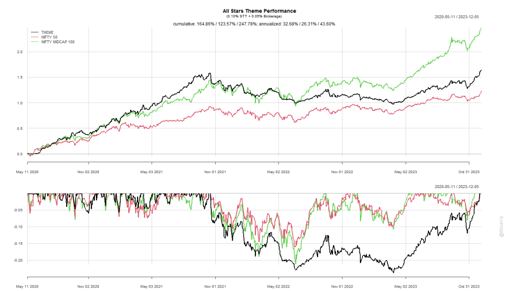
For example, our All Stars strategy recently hit a Sharpe of 2.0, which is sort of a holy grail in investing. However, if you had looked at it a few months ago, when it was still recovering from a drawdown, you would’ve stayed clear of it. So, what changed? The everything rally in stocks.
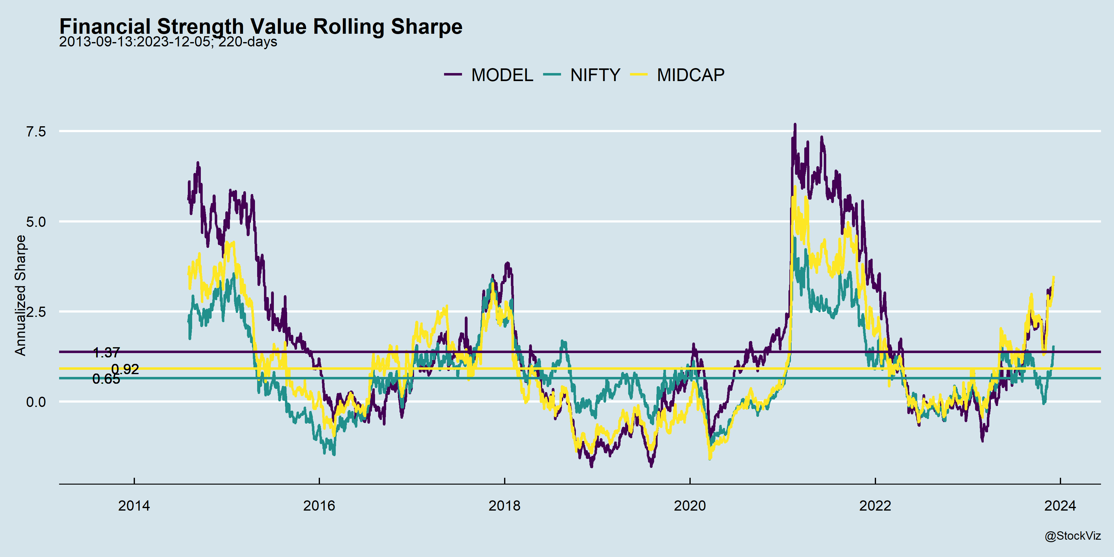
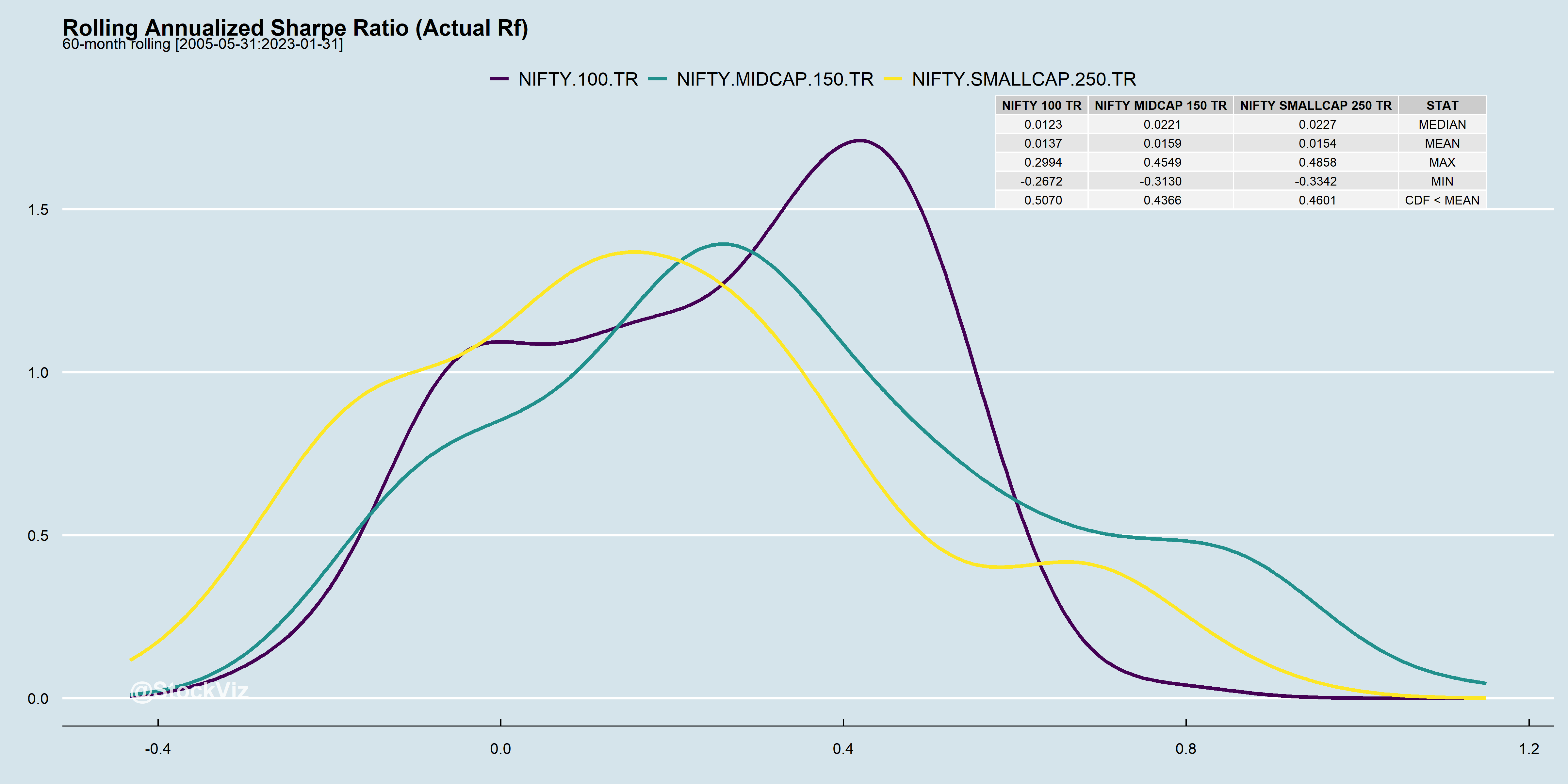
One way to avoid falling into this trap is to also look at the rolling Sharpe ratio over the life of the strategy.
While this is particularly true for momentum strategies that all look exceptional in bull markets, value strategies are not immune to this effect either.
Lifetime metrics are also sensitive to launch dates as well. Long running strategies would’ve seen their fair share of market ups and downs compared to newer ones launched during bear markets.
Rolling metrics will help investors get a better idea about strategy performance.
Sharpe Ratios are often used to sort through competing investments. It is the original “risk adjusted returns.” It’s a mathematical expression of the insight that excess returns over a period of time may signify more volatility and risk, rather than investing skill (investopedia, wikipedia).
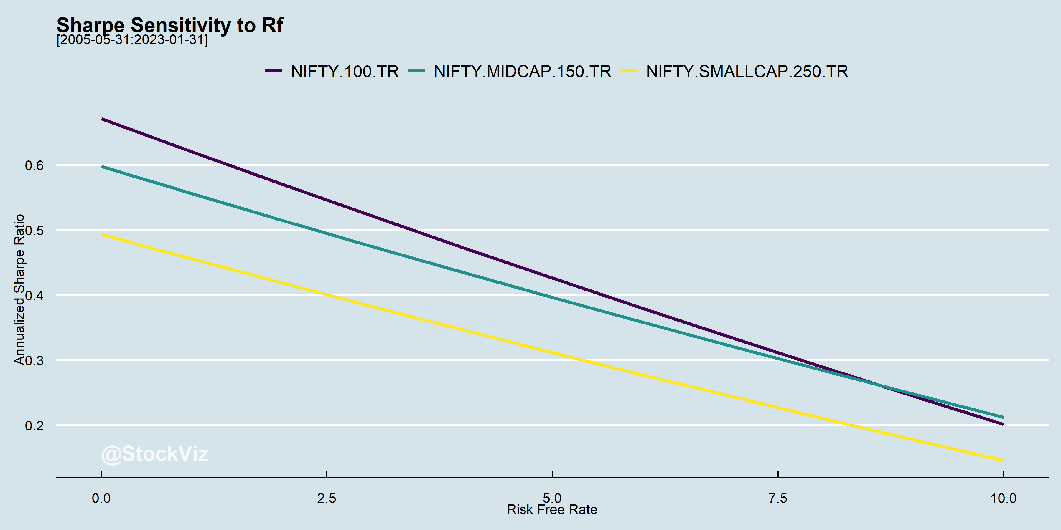
Rb or Rf, the risk-free return, is usually cumbersome to handle. So, typically, it is either set to zero or a constant value. The problem is that rates vary over time and has an impact on the relative ordering of investments.
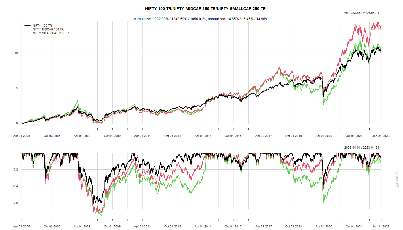
At high interest rates, SR(mid-caps) > SR(large-caps)
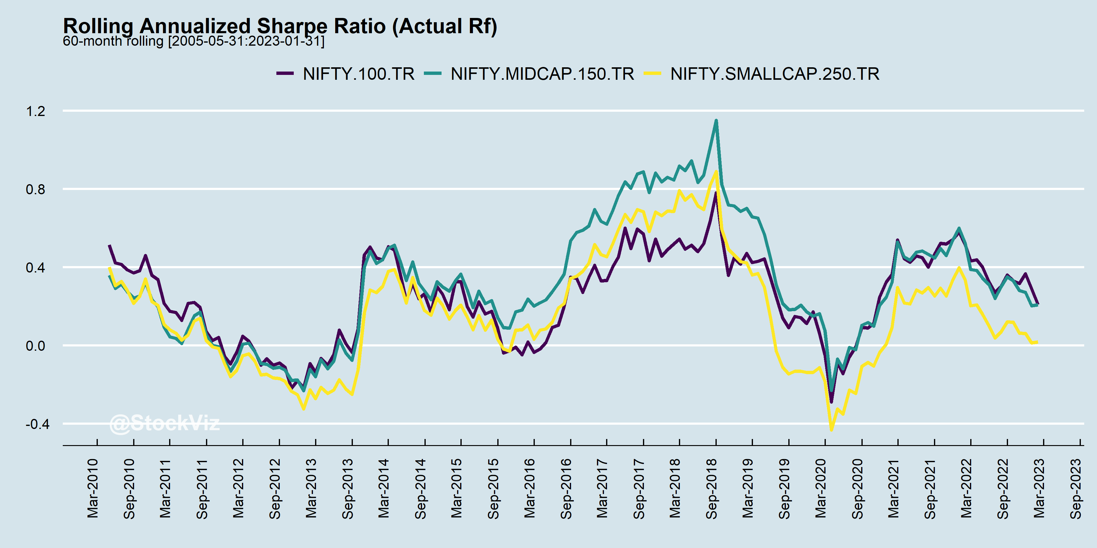
Ideally, you want your Sharpes to be positive and stable. Unfortunately, that is never the case.
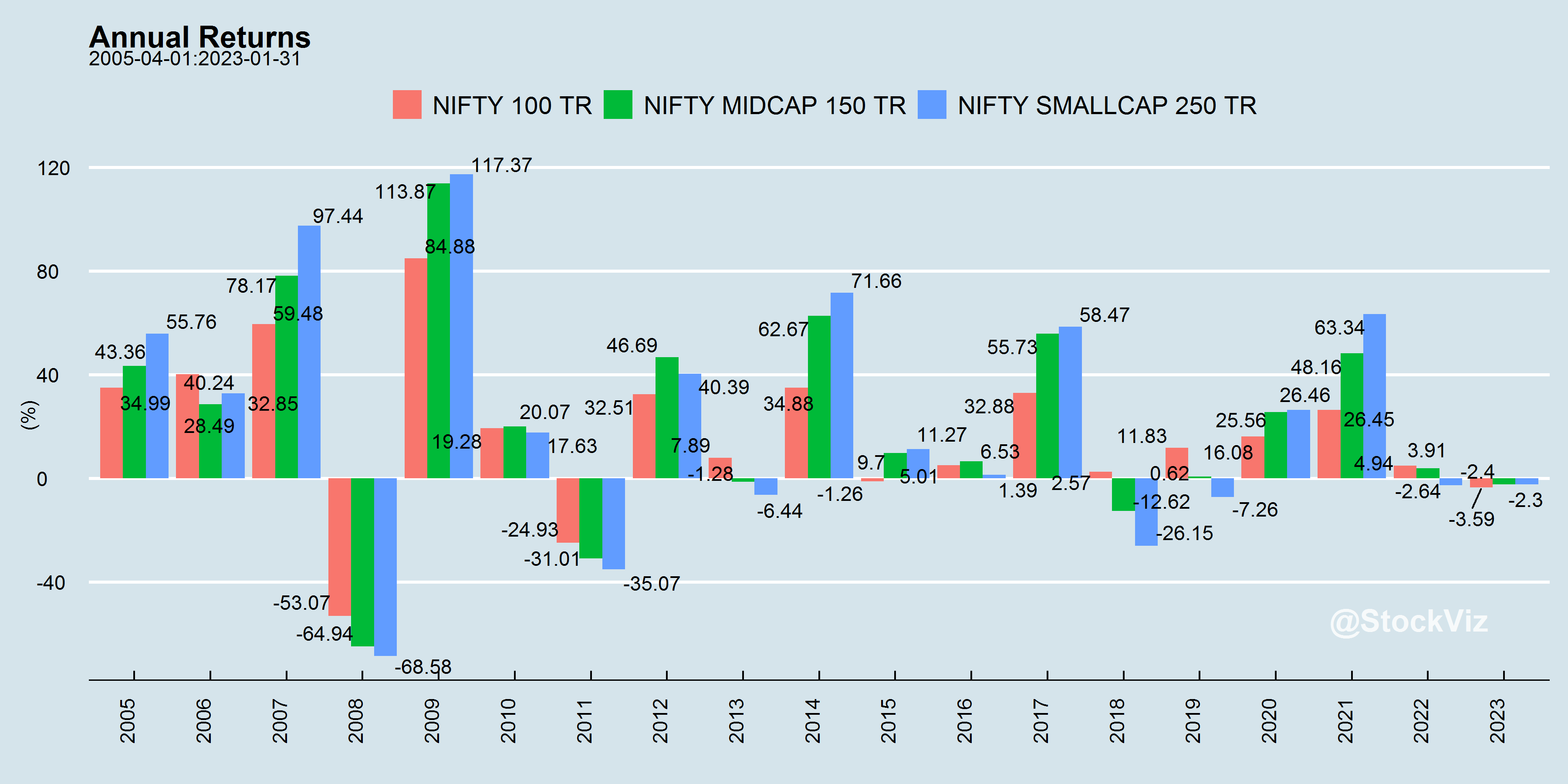
During bull markets, Sharpes trend up and reverse course in bears.
At the end of the day, it boils down to whether the returns are worth the risk.
You might very well be trying to catch lightening in a bottle.
For more index stats, visit our Index Metrics dashboard.
In our introduction to factors, we discussed how portfolio returns are mostly explained by market risk (rm – rf: market risk premium.) Whatever cannot be explained by the market is α, or the portfolio manager’s skill. If you strip away the financial jargon, this is nothing but linear regression.
Also, what exactly is “market risk?” A few years ago, the only index funds on the market were of the NIFTY 50 and MIDCAP 150 indices. However, the number of index funds keep ticking up and there are now several strategy funds covering quality, value, low-volatility, momentum, etc… in the market. So, if an investor can access these vanilla strategies at a low cost, shouldn’t the definition of the “market” expand to incorporate those?
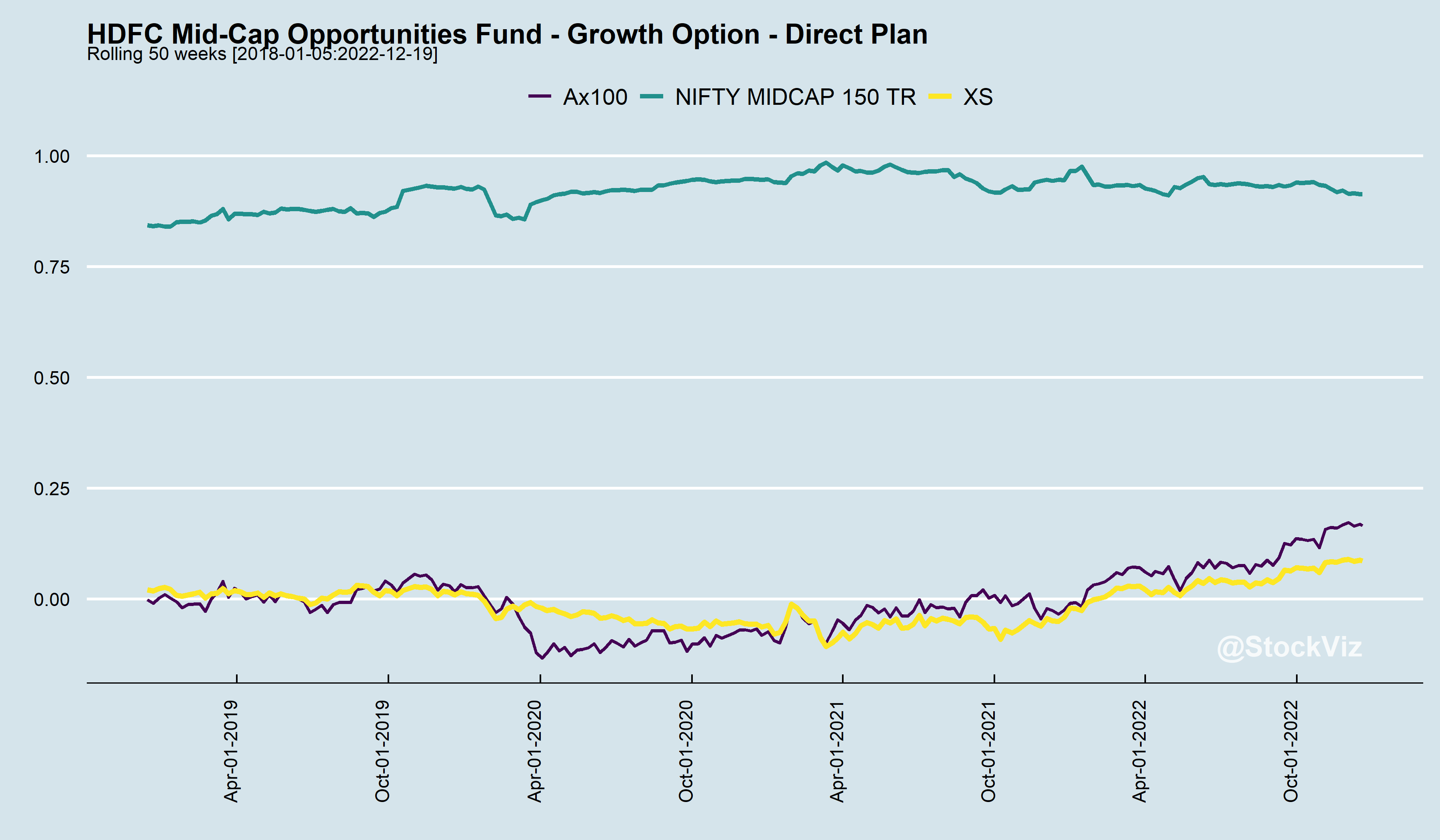
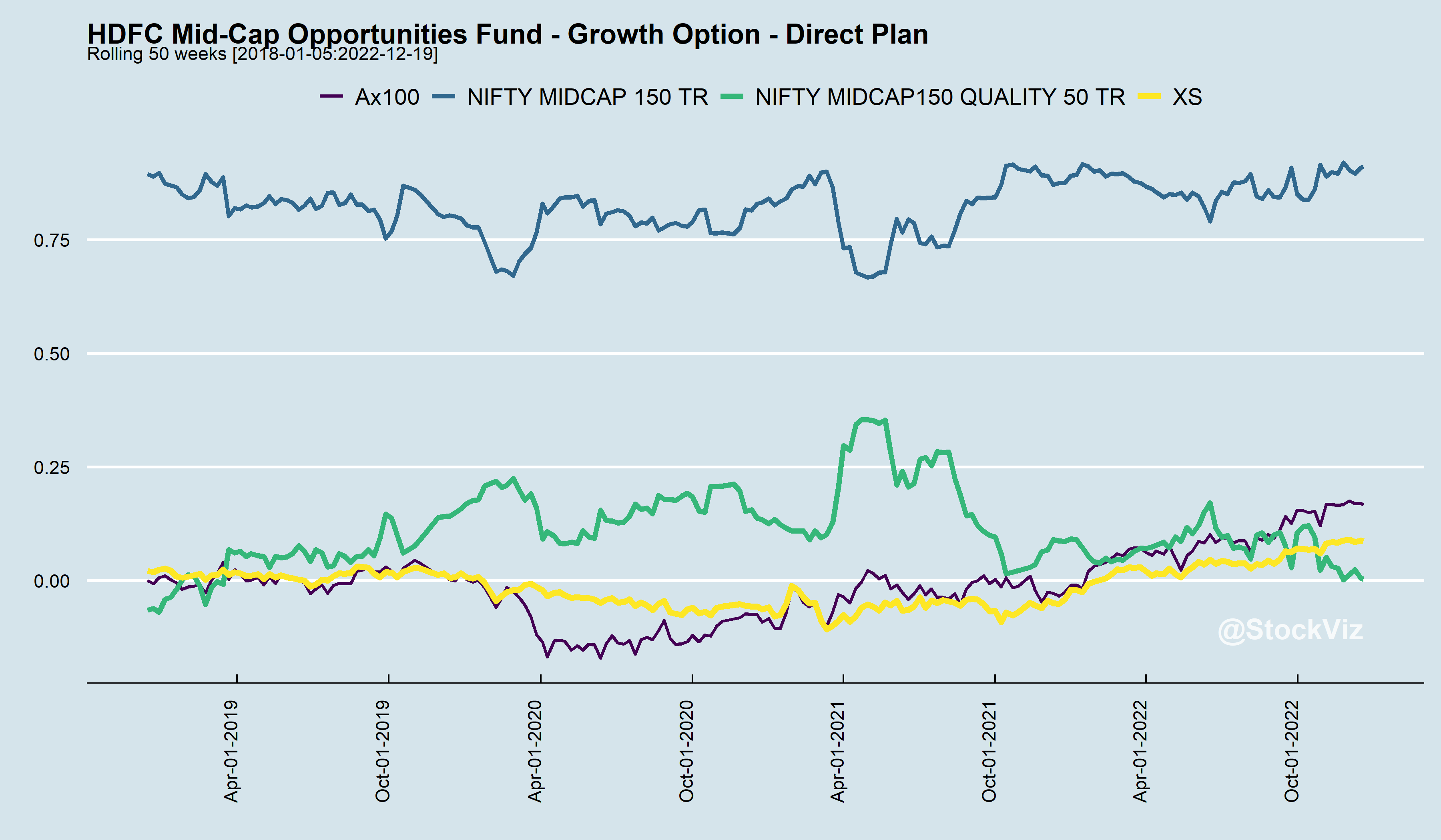
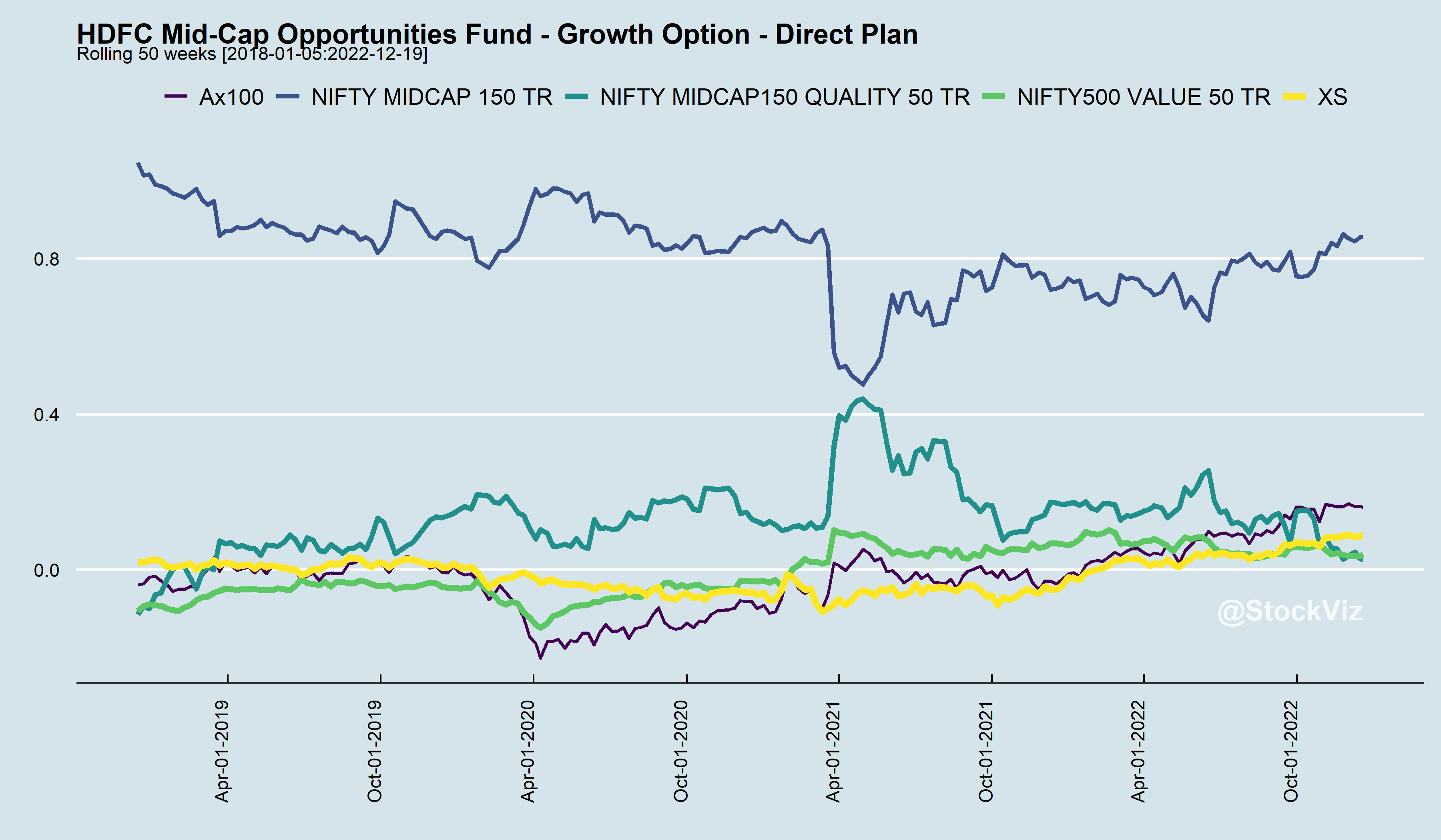
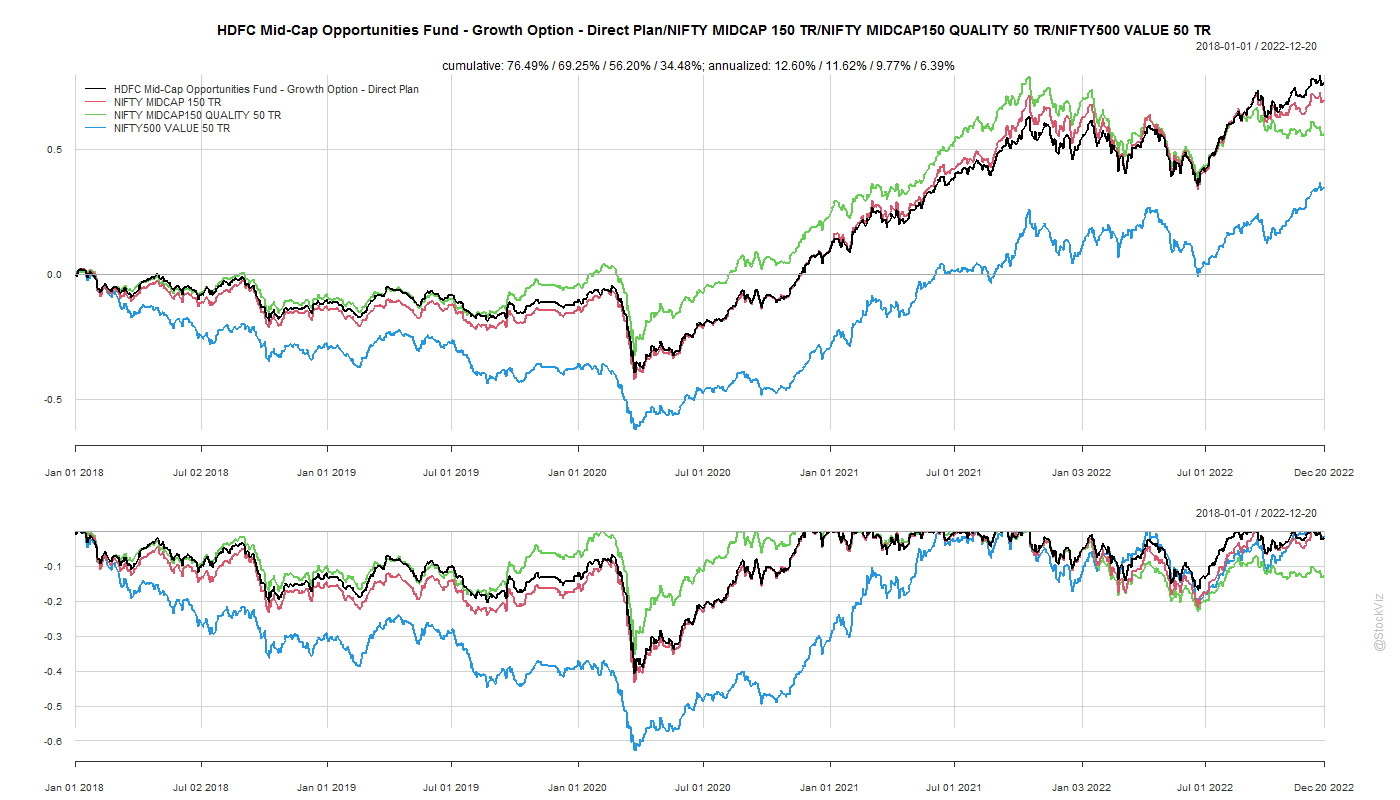
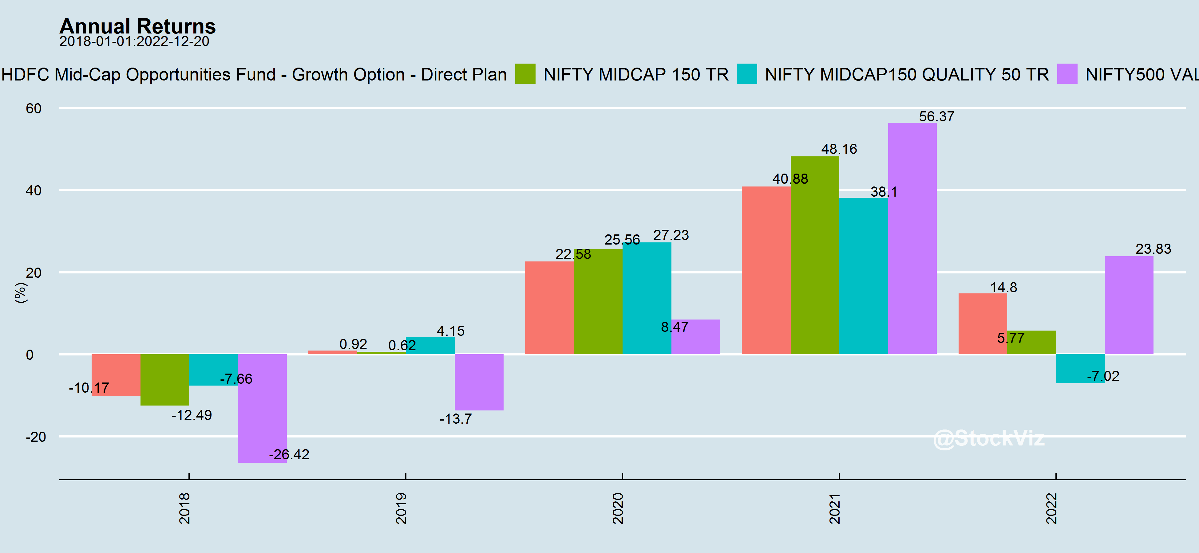
For example, take the HDFC Mid-cap Opp. Fund. You could regress its returns against the NIFTY MIDCAP 150, the NIFTY MIDCAP150 QUALITY 50 and NIFTY500 VALUE 50 indices to get an idea of how its α over them has evolved over time.
Rolling regressions gives you an idea of portfolio tilts and the fluctuating nature of α (Ax100). Also, its worth noting that α is only tangentially related to excess returns (XS). There are periods here where XS was positive in spite of negative Ax100 and vice versa.
Styles go in-and-out of favor. Sometimes Quality performs better than Value and sometimes a simple cap-weighted index will outperform everything else. An actively managed portfolio’s relative performance to these styles change over time as well.
tl;dr:
α is a statistical derivation.
Don’t go chasing α – it keeps fluctuating.
α is not the same as excess returns.
When in doubt, index and forget.
You are always in doubt.
We have setup a script that auto-updates every day with these regressions on select large-cap and mid-cap funds. The report is available here.
First time investors often get bedazzled by tall claims of “20%” returns in direct equities. All they need to do is subscribe to an “exclusive” telegram channel or advisory service and mint their way to millions. Even if these claims were true, gross returns – the number often marketed – has little to do with the net returns that the investor finally realizes at the end of the year.
Very few know that a high-churn portfolio that delivers 20% gross returns is equivalent to a mutual fund that delivers 14% net. So, who ate your cheese?
Layers of Transaction Taxes
Securities Transaction Tax (STT)
The STT is an automatic tax collected by the government on all transactions irrespective of whether you made money on it or not. On equities, it is currently set at 0.1% – if you bought & sold 1 stock worth Rs. 100, then the government collects 20p on it. This is one of the biggest drags on high-churn strategies.
Last year, the government collected ₹16,927 crore in STT.1
Exchange Transaction Charges
The trading venue, typically the NSE (National Stock Exchange) or the BSE (Bombay Stock Exchange,) levies a transaction charge for allowing you to trade through them. This varies by exchange and they are know to give rebates to high volume brokers to keep them loyal. The last time I checked, it was around 0.00345% on the NSE.2
Stamp Duty
When the Central Government is skimming off through STT, why should State Governments be far behind? The states too have their hands in the till through “stamp duty.”
Stamp duty is a state levy paid to register a document, typically an agreement or transaction paper between two or more parties, with the registrar. In an era where all transactions are electronic and registering transactions is just flipping some bits in a database, this is basically free money to the states.
Before 2020, every state had its own rate but thankfully, the Modi Government rationalized it to a common rate of 0.015% on the buy-side of equities.3
SEBI Turnover fees
If you though that SEBI was an arm of the government and should be entirely funded by the general budget, the joke is on you. If you have a look at your contract note that the brokers sends you on the days that you trade, you’ll find a “SEBI Turnover Fee.” This is 0.00015% on both buys & sells. While its one of the smaller taxes/fees on transactions, it is still a percentage of total volume, so it adds up over time.4
During 2019-20, the total amount of fees and other charges collected by SEBI was Rs. 608.26 crore.5
Short-term and Long-term Capital Gains Tax
The rationale behind STT, introduced in 2014, was to replace the long-term capital gains tax. It was said that there was a lot of “leakage” in collecting LTCG and that a tax on transactions collected directly by the exchanges would plug it. However, the 2018 budget saw the re-imposition of LTCG.6
However, if your strategy demands churn, then you need to be worried more about STCG (15% on profits) than on LTCG (10% on profits.)
A High Bar of Direct-Equity
After all these taxes, levies and charges, when the numbers are tallied up at the end of the year, most direct-equity investors would be better off with a mutual fund.
The napkin math (sheet) above doesn’t consider brokerage – since those are mostly zero – and DMAT charges – those charged by CDSL – since those are flat fees charged only on sales.
Direct-equity investing strategies need to walk a fine line between optimizing for lower transaction costs, risk management and taxes. This is where we find advisory disclosures lacking. Most advisors do not disclose portfolio churn rates and nor do they indicate what the net, after-tax, returns would look like.
Also, a mutual fund’s NAV includes all of these charges and your portfolio compounds tax-free until you redeem. So, if you have a 5+ year time horizon, then compounding the 15% STCG adds significant tailwinds to your portfolio.
Conclusion
While comparing different strategies, investors should also consider portfolio churn and try and back into what the net, after-tax, returns would look like at the end of the year. Know that mutual fund NAVs are net of transaction costs and can compound tax-free.
Direct-equity strategies should clear a high-bar.
Looking for a sensible way to invest? Here’s how to get started.