First came the market, then came the factors…
The Efficient Market Hypothesis
Two economists walk down a road and they see a twenty dollar bill lying on the side-walk. One of them asks “is that a twenty dollar bill?” Then the other one answers “It can’t be, because someone would have picked it up already,” and they keep walking. (source)
In 1965, Eugene Fama published his dissertation arguing for the random walk hypothesis. i.e., stock market prices evolve according to a random walk (so price changes are random) and thus cannot be predicted. This was followed by Paul Samuelson, who published a proof showing that if the market is efficient, prices will exhibit random-walk behavior. (source)
Together, they form the basis of the efficient market hypothesis (EMH).
The efficient market hypothesis (EMH), is a hypothesis that states that share prices reflect all information and consistent alpha generation is impossible. According to the EMH, stocks always trade at their fair value on exchanges, making it impossible for investors to purchase undervalued stocks or sell stocks for inflated prices. Therefore, it should be impossible to outperform the overall market through expert stock selection or market timing, and the only way an investor can obtain higher returns is by purchasing riskier investments. (source)
Inefficiencies are opportunities
Any market practitioner knows that this is not entirely true. There are numerous hurdles in the way of pure efficiency:
Information is not free.
Liquidity is not unlimited.
Prices are not continuous.
Market statistics are forever in flux.
Investors have different goals and pursue different outcomes.
Taxes, rules and regulations.
According to EMH, a portfolio’s return could be fully explained by the market (source):
r = rf+ ß(rm – rf) + α
Where:
r = Expected rate of return
rf = Risk-free rate
ß = Beta
(rm – rf)= Market risk premium
This is a single-factor model. i.e., portfolio returns are only explained by market risk (rm – rf: market risk premium.) Whatever cannot be explained by the market is α, or the portfolio manager’s skill.
However, if you setup a portfolio in certain ways, you consistently ended up with higher returns, implying that there was something about the market, something systematic, that was not being captured by this equation. So, if you were rewarding a portfolio manager only on the basis of α calculated from the above equation, then you were probably over-paying the PM for harvesting something that the market offered for “free.”
In 1992, Eugene Fama and Kenneth French designed a model to fix this – the Fama–French three-factor model.
The Fama-French model aims to describe stock returns through three factors: (1) market risk (rm – rf: market risk premium,) (2) the outperformance of small-cap companies relative to large-cap companies (SMB: Small Minus Big,) and (3) the outperformance of high book-to-market value companies versus low book-to-market value companies (HML: High Minus Low.) The rationale behind the model is that high value and small-cap companies tend to regularly outperform the overall market. (source)

Where:
r= Expected rate of return
rf = Risk-free rate
ß = Factor’s coefficient (sensitivity)
(rm – rf)= Market risk premium
SMB(Small Minus Big) = Historic excess returns of small-cap companies over large-cap companies
HML(High Minus Low) = Historic excess returns of value stocks (high book-to-price ratio) over growth stocks (low book-to-price ratio)
↋= Risk, or α
Think of SMB and HML as “base-rates.” A portfolio’s returns can now be explained by the degree of tilt (factor cofficients, ßs) it has towards value (HML) and small-caps (SMB). Furthermore, you can set up incentives for the portfolio manager that incorporates these factors so that he is rewarded only if he can out-perform a generic small-cap/value portfolio.
The academic definition of value (HML) and small-caps (SMB) is quite different from what investors are used to colloquially. Fama and French were interested in the decomposition of portfolio returns into sub-components (factors) and the persistence of these factors over many years/decades. They did this by constructing SMB and HML as long-short portfolios and analyzing the spread. It is very different from what the media refers to by these terms. It is useful to think of these as spreads and not as typical long-only “value” portfolio.
No pain, No gain
Just because these factors are persistent, doesn’t mean that they are always positive. A simple way to visualize this is to see the cumulative returns of the market risk premium (MKT = rm – rf) over SMB and HML.
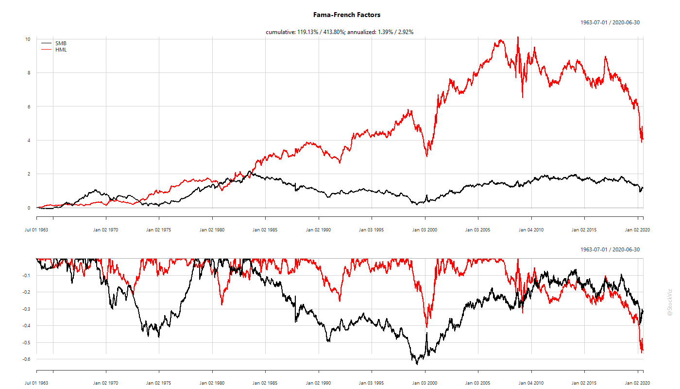
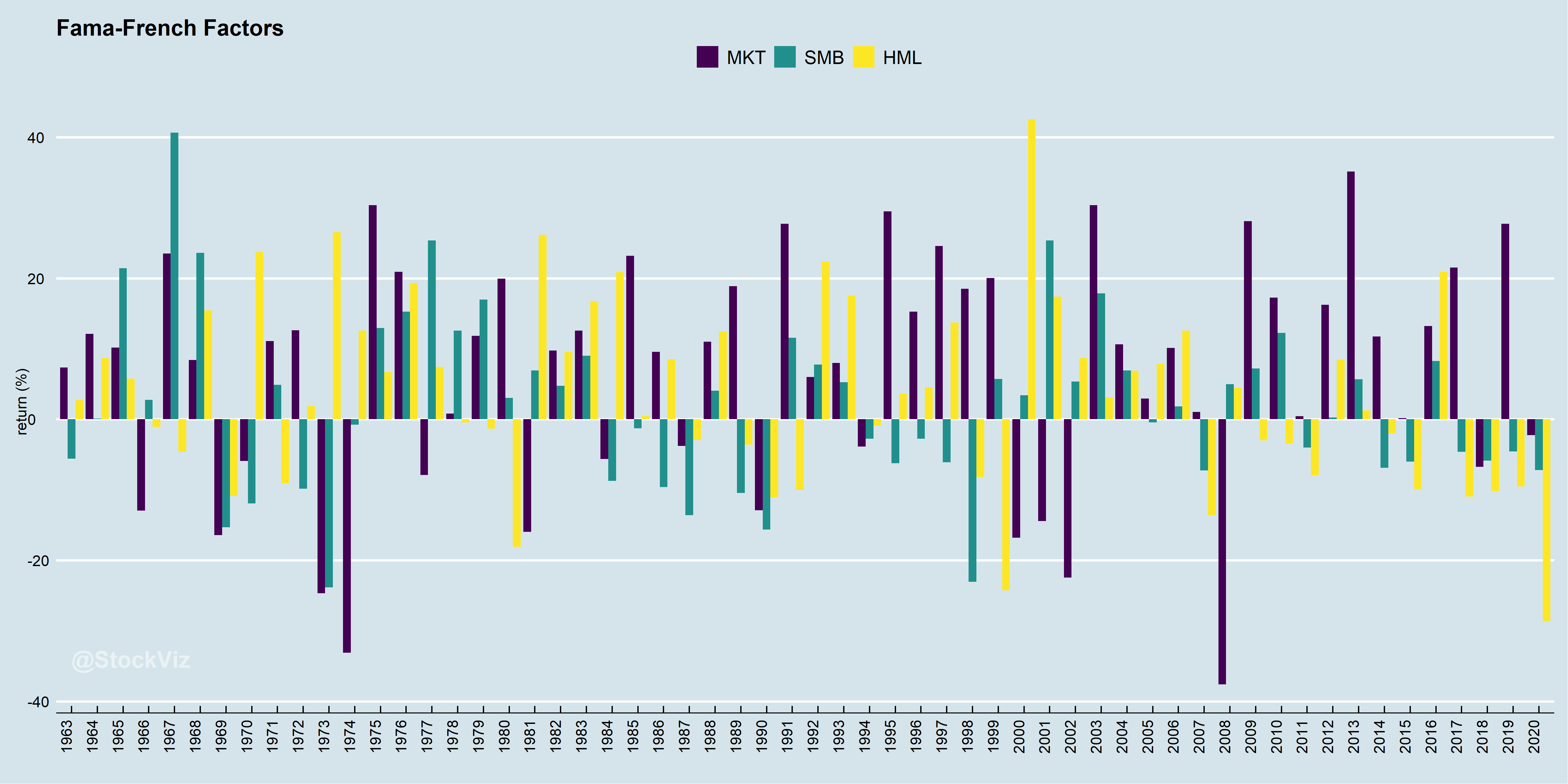
There are periods of both out-performance and under-performance. In fact, one of the theories proposed to explain the persistence of these factors is behavioral: investors herd into value or small-caps based on recent out-performance. Thus, setting them up for subsequent under-performance. Upon which, they will exit en masse, allowing the factors to out-perform once again.
The real world is messy
Most investors are long-only. Whey we buy a value fund, for example, we are not really buying a Fama-French HML long-short portfolio. Our portfolios have a market beta and a bunch of other things affecting it besides high book-to-price ratio.
To visualize this, if we decompose the iShares Russell 1000 Value ETF, IWD, to its 3-factors, we get:
rf + 0.92*(rm – rf) – 0.06*SMB + 0.35*HML + α
Compared to iShares Russell 1000 Growth ETF, IWF:
rf + 1.03*(rm – rf) – 0.05*SMB – 0.27*HML + α
Conclusion
The Fama-French 3-Factor model is a useful tool to analyze investment portfolios. It allows us to decompose returns to different factors so that we can better understand the drivers of returns.
Coming up next: The Fama-French 5-Factor model.
Enjoy our discussion: