When you use the Black-Scholes-Merton (BSM) model, you end up with theoretical prices that assumes that volatility affects all strikes uniformly. i.e., strikes have no bearing on implied volatility (IV). This was largely true in the market as well until the crash of 1987. However, after the October 1987 crash, the implied volatility computed from option prices using the BSM model started differing between puts and calls. This is called “volatility smile“, or the smirk, given its actual shape.
The reason for this is quite simple, markets take the stairs up and the elevator down. Fat tails, if you must. So, put options sellers require a little bit of an incentive to take on that risk.
How crooked is the smirk? If you take the ratio of the IVs of OTM puts to OTM calls and plot them, you’ll notice that as you get farther away from spot, the distribution flattens out.
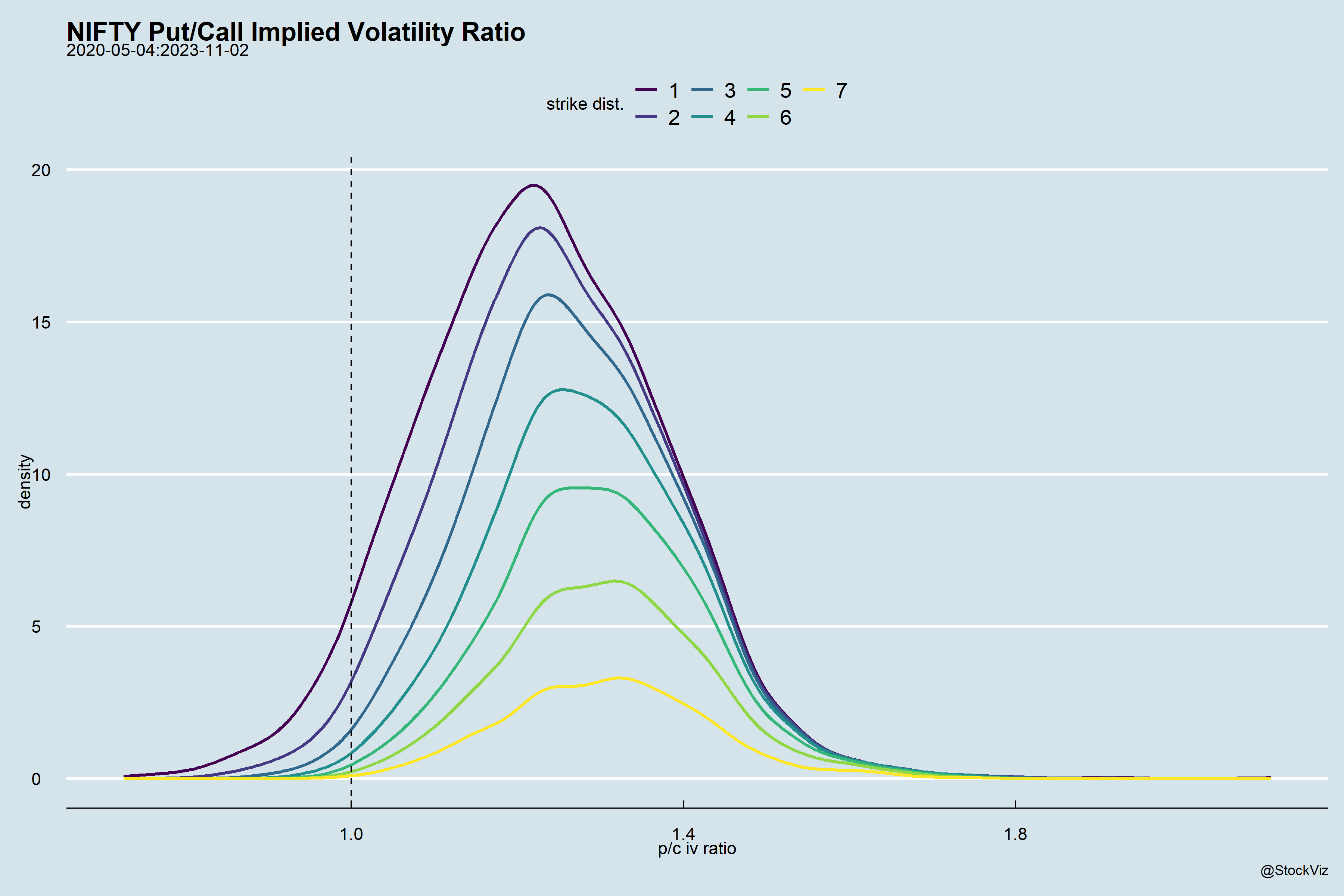
Notice the area below 1.0? Those are the days when the calls were trading at a higher IV than the puts.
On the left of zero are the calls with descending order of strikes and on the right are puts with ascending order of strikes. The farther away from zero, the more OTM they are.
Also, unlike the stylized charts of IV you might have seen with sweet smiles, the reality is quite different.

If this tickles your curiosity, do read The Risk-Reversal Premium, Hull and Sinclair (SSRN)
Code and charts on github.