A lot of ink is spilled on the budget. Some are prescriptive (and completely useless.) Some are predictive (and mostly wrong.) Most investors will do well to just ignore the noise and continue with their SIP/DCA. However, if you do want to trade it, what should you do?
Of the last 26 budgets, 16 ended the day red. You could just short the NIFTY and play the odds.
Budget days tend to have huge intraday ranges that lead to dislocations that you could monetize. However, this is largely a high-frequency trading affair and may not be feasible for most.
Another thing worth pursuing are delta-hedged short-strangles. The table above gives you the P&L of shorting NIFTY ATM delta-hedged strangles overnight and closing them on budget-day (or the immediate business-day.) There’s a fair amount of execution risk here given the intraday volatility on the day. However, it seems like a decent profit pool to fish in.
While the concept of volatility smirk is simple, the pattern itself is unstable. For example, different expiries have different shapes.
And these shapes change across days as well.
One way to keep track of these changes is by fitting a model through the implied volatilities. Here, we fit a parabola (y = ax2 + bx + c). a, the coefficient of strike_pct2, gives a measure of the narrowness/steepness of the smirk.
By sampling the curve and tracking these coefficients, you can begin to form an opinion on what is “normal” vs. a trading opportunity.
The volatility risk premium (VRP) is the difference between implied volatility and realized (or actual historical) volatility. Implied volatility is, on average, overpriced compared to realized volatility.
The VRP exists because investors are essentially “selling insurance” when they sell implied volatility.
Volatility is negatively correlated with equity returns; typically, volatility increases when equity markets decline. Therefore, a short volatility position is implicitly “long equity risk”. Since equities are generally expected to earn an equity risk premium (ERP) over the risk-free rate, strategies that are implicitly long equity risk should also be abnormally profitable. This is why short volatility strategies tend to be profitable on average.
Just like how you can get long ERP by getting long an equity index, you should be able to get long VRP by programmatically shorting options and delta-hedging them. Volatility becomes a beta that you allocate towards.
Building Blocks
An option’s value changes relative to the price of the underlying – the rate of this change is called delta.
Gamma is the rate of change of delta given a change in the price of the underlying. As the underlying price moves, an option’s delta does not remain constant; gamma quantifies how much that delta will change.
Since we are only interested in volatility and not price, we can hedge out this delta. Delta-hedging a basket of options mitigates the exposure to the directional movement of the underlying. Profitability becomes solely determined by the volatility (not direction) of the underlying.
Vega is the rate of change of an option’s value relative to a change in implied volatility (IV). If IV rises or declines by one percentage point, the value of the option is expected to rise or decline by the amount of the option’s vega, respectively.
When you short options, you have negative gamma (you don’t want large price movements) and negative vega (you don’t want IV to rise). You hope for low realized volatility and falling IV. However, you have positive theta — time works in your favor.
Theoretically, a delta-hedged short option position’s P&L = vega(IV – RV).1
Construction
Historically, NIFTY ATM option Implied Volatility across days-to-expiry, looks like this:
So, theoretically, if you shorted 30dte ATM calls and exited them at 7dte, your P&L distribution will look like this:
And the same thing with puts:
If you are willing to treat volatility as just-an-other beta, then by creating programmatic delta-hedged short ATM straddle/strangle portfolio, you can get long this beta.
Just as it is with ERP, one could build models to time VRP. Having a beta portfolio as a benchmark should help.
When you use the Black-Scholes-Merton (BSM) model, you end up with theoretical prices that assumes that volatility affects all strikes uniformly. i.e., strikes have no bearing on implied volatility (IV). This was largely true in the market as well until the crash of 1987. However, after the October 1987 crash, the implied volatility computed from option prices using the BSM model started differing between puts and calls. This is called “volatility smile“, or the smirk, given its actual shape.
The reason for this is quite simple, markets take the stairs up and the elevator down. Fat tails, if you must. So, put options sellers require a little bit of an incentive to take on that risk.
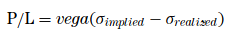
How crooked is the smirk? If you take the ratio of the IVs of OTM puts to OTM calls and plot them, you’ll notice that as you get farther away from spot, the distribution flattens out.
Notice the area below 1.0? Those are the days when the calls were trading at a higher IV than the puts.
On the left of zero are the calls with descending order of strikes and on the right are puts with ascending order of strikes. The farther away from zero, the more OTM they are.
Also, unlike the stylized charts of IV you might have seen with sweet smiles, the reality is quite different.
If this tickles your curiosity, do read The Risk-Reversal Premium, Hull and Sinclair (SSRN)
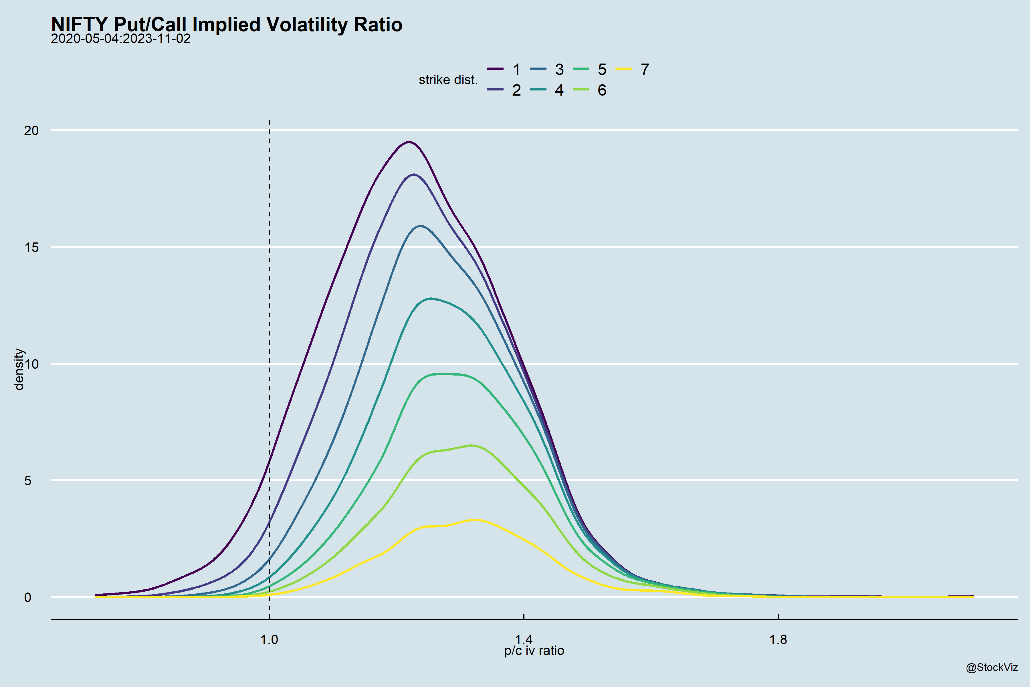
Summary: Mar NIFTY 18000 calls added 65,14,850 contracts while 17400 calls shed 44,21,500. On the Put side of the equation, the 17500 strike added 80,10,000 while the 16850’s shed 4,60,800.
MAR NIFTY OI
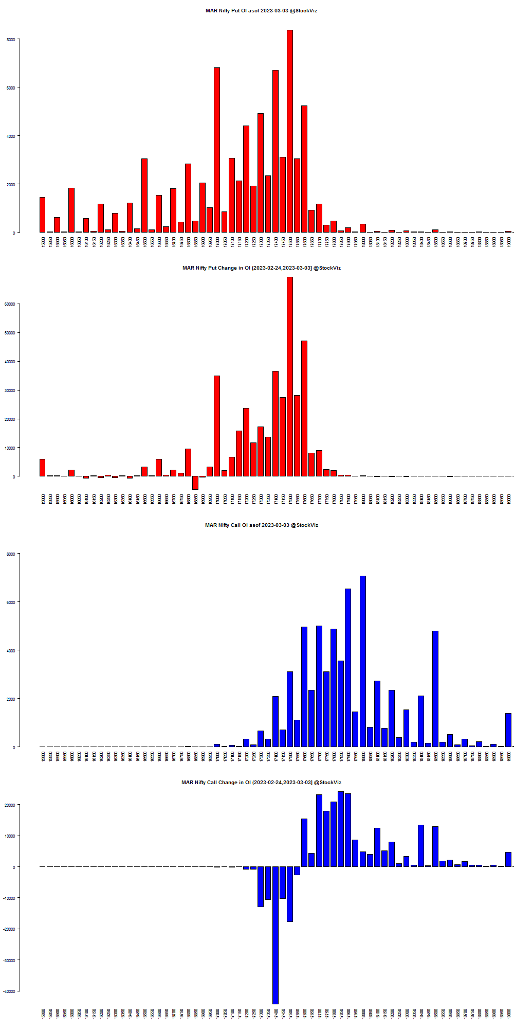
MAR BANKNIFTY OI
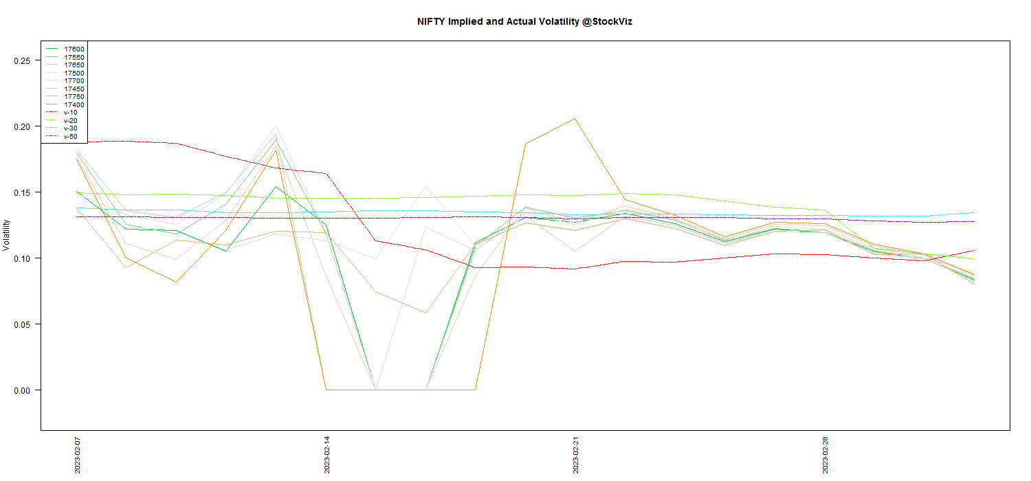
MAR NIFTY Volatility
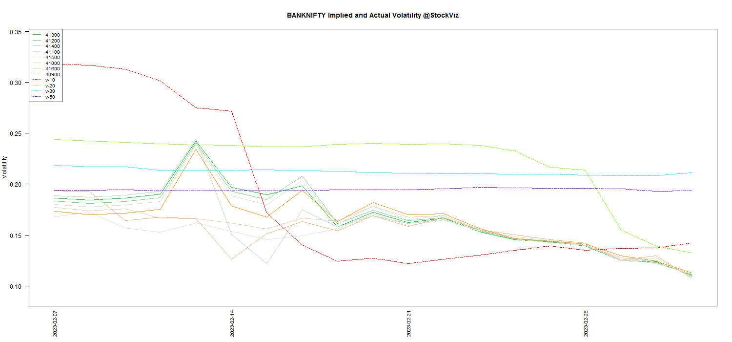
MAR BANKNIFTY Volatility
Dotted lines indicated actual underlying volatility. Solid lines are IVs.