Tag: momentum

Reducing Crash Risk in the Nifty Alpha Indices

shyam November 21, 2019October 27, 2020

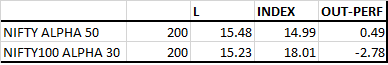
The NSE has a couple of strategy indices – the NIFTY Alpha 50 Index and the NIFTY100 Alpha 30 Index – based on historical CAPM alphas. The former selects 50 stocks from the largest 300 stocks whereas the latter selects 30 stocks from the NIFTY 100 index.

First, a look at a simple buy-and-hold strategy.

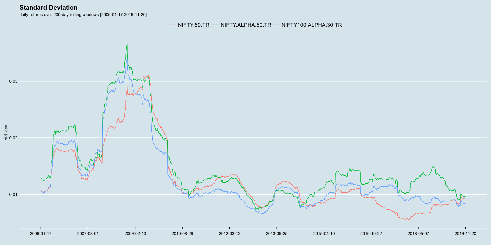
Buy-and-Hold Curves

NIFTY ALPHA 50 TR vs NIFTY100 ALPHA 30 TR

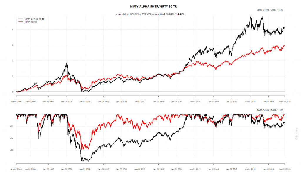
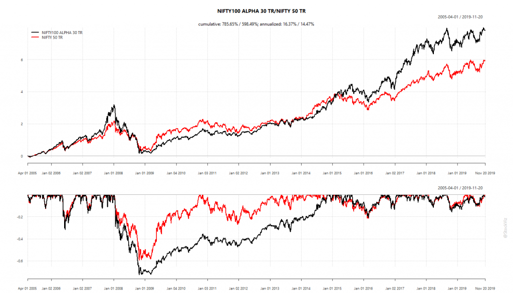
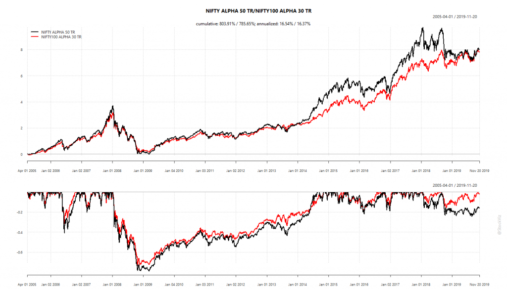
The alpha indices have out-performed the plain-vanilla NIFTY 50. However, what jumps out off the page is the sheer depth and length of the drawdows that these indices have made.

Even though they give vastly better returns than the NIFTY 50 index, the lived experience would be too painful for most investors. Is there a way to reduce these drawdowns while retaining most of the out-performance?

In a 2012 paper, Momentum has its moments, Barroso and Santa-Clara outline a way in which historical volatility could be used to reduce momentum crashes.

Strategy Outline

The basic idea is that momentum risk is time-varying and sticky. And, periods of high risk are followed by low returns.

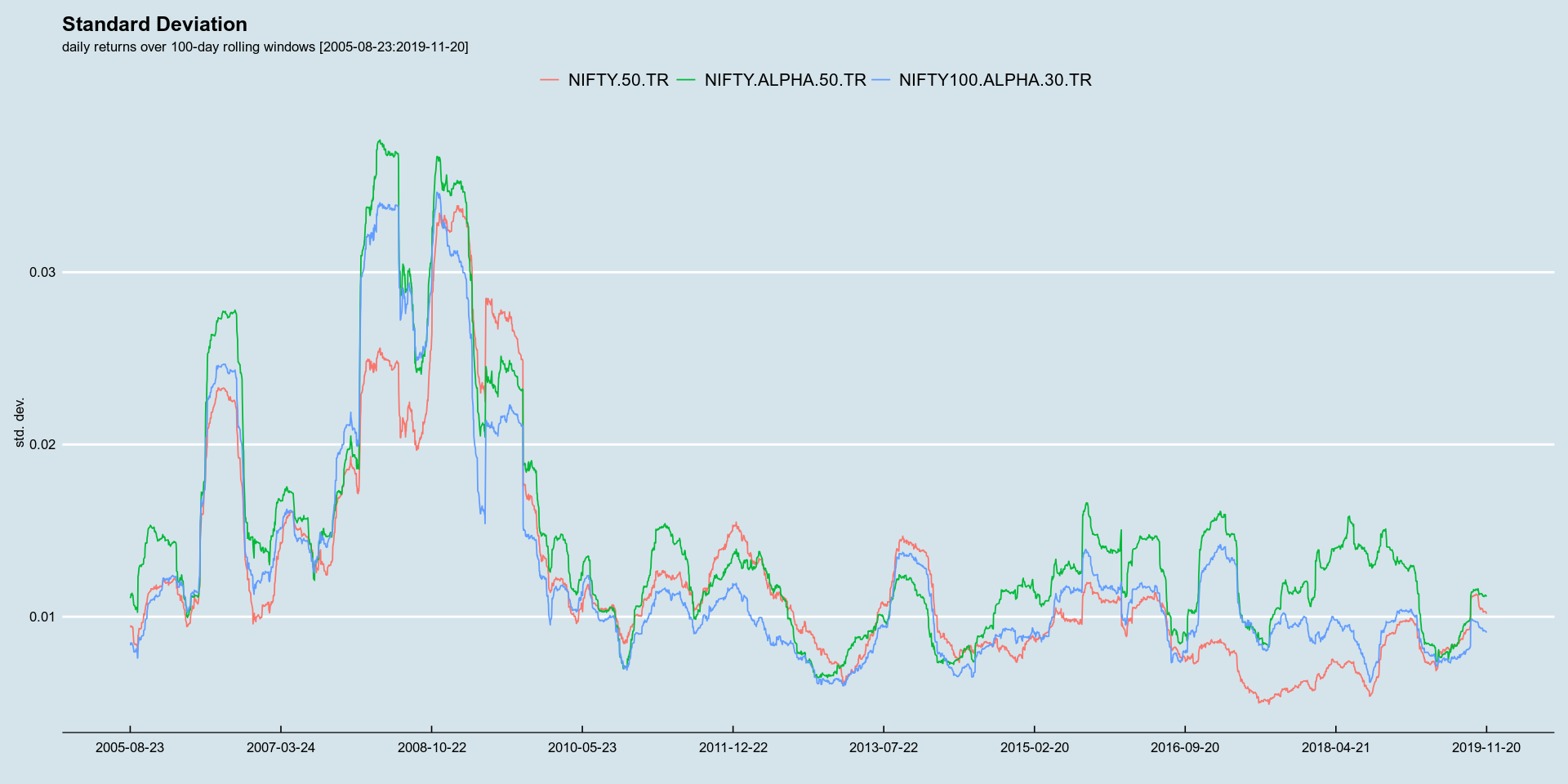
To test this theory out on the Alpha indices, we first split the time series into halves. The first to “train” and the second to “test.” We need a training set because we are not sure what the appropriate look-back for calculating risk should be (we check 100- and 200-days). The test set is a check of out-of-sample behavior of the strategy.

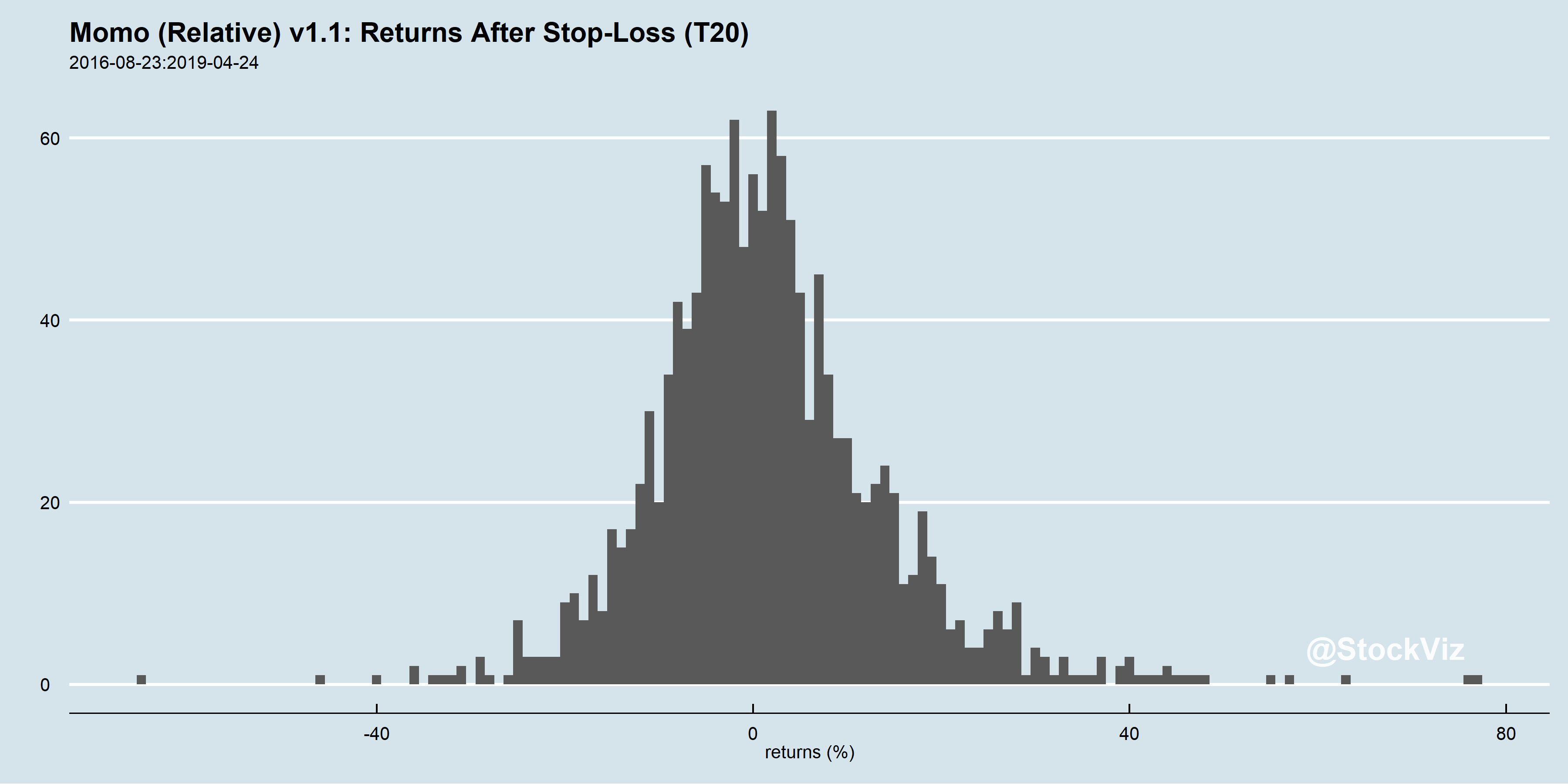
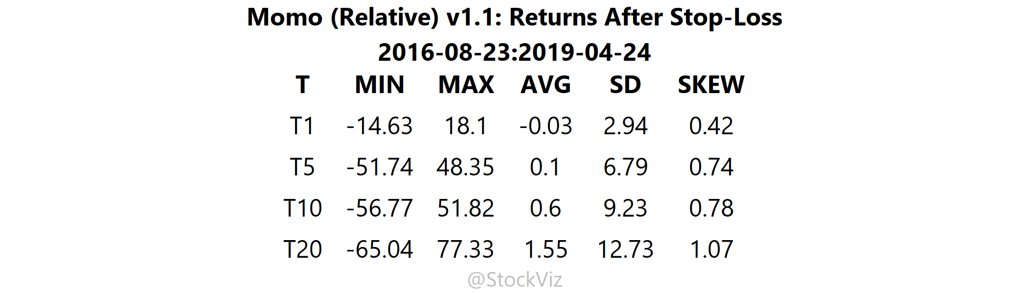
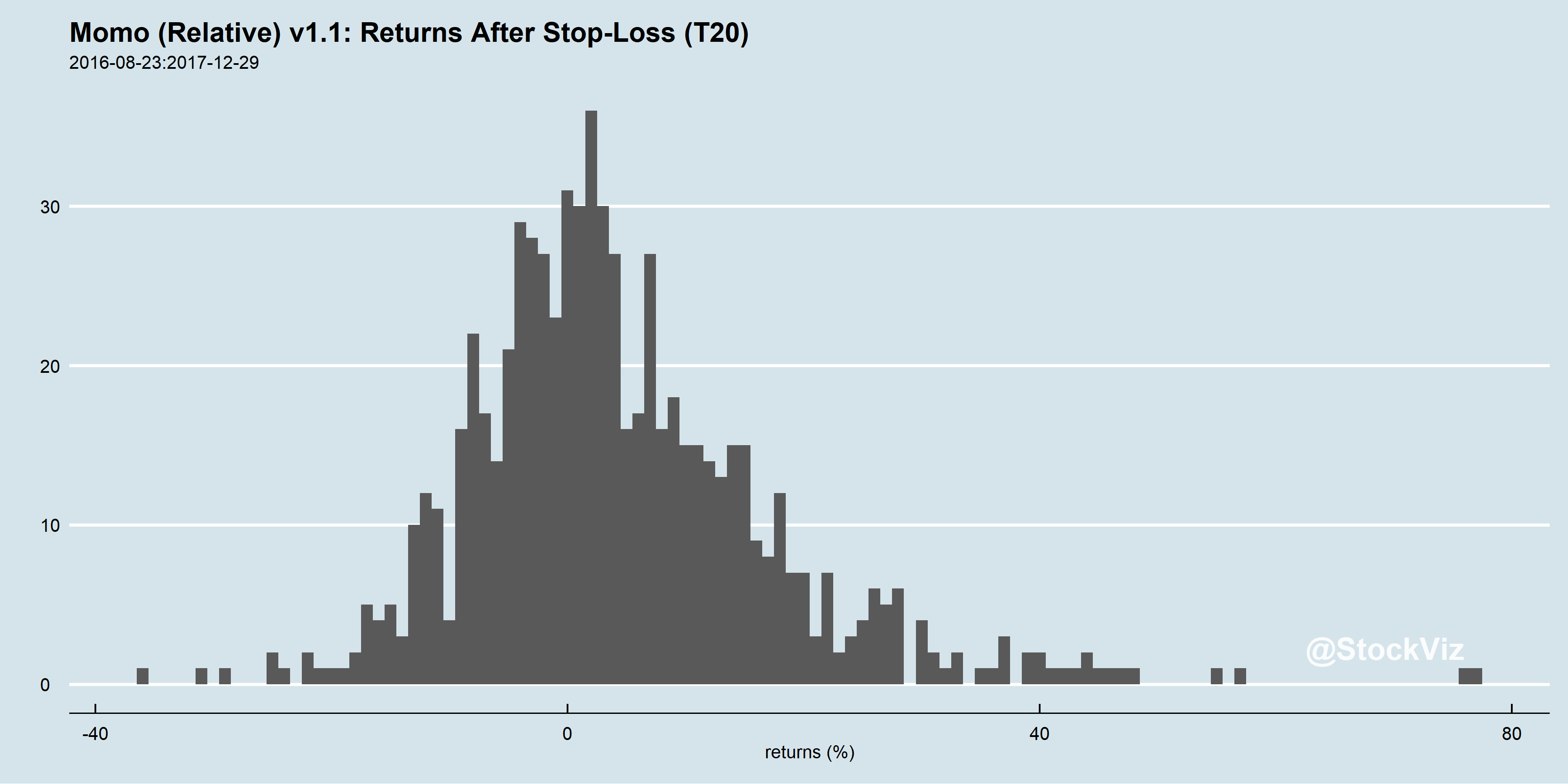
The theory laid out in the paper, that periods of high risk is followed by periods of low returns, is true. Subsequent returns when std. dev. is in the bottom deciles show large negative bias. Also, perhaps indicating a bit of mean-reversion, returns after std. dev. is in the 7-9th decile, have fat right tails.

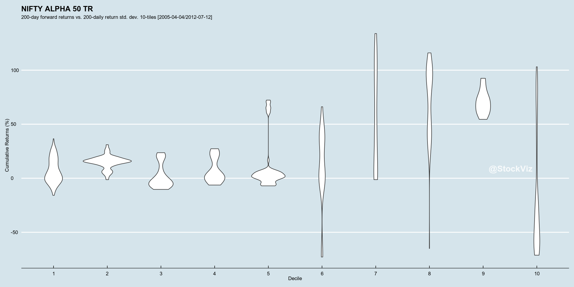
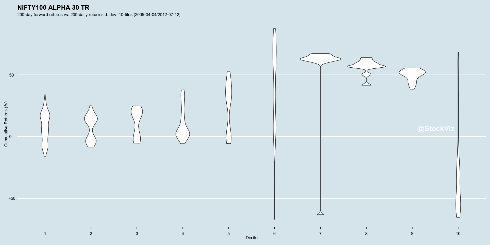
NIFTY ALPHA 50 200-day cumulative returns by 200-day sd decile

NIFTY100 ALPHA 30 200-day cumulative returns by 200-day sd decile

Train In-Sample

The next question is the appropriate lookback and deciles for calculating the std. dev. Running this on the training set, we find:

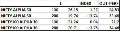
A strategy that goes long Alpha when std. dev. is in the 1-5 deciles side-steps severe drawdowns in the training set. Note, however, that it under-performed buy-and-hold during the melt-up of 2007.

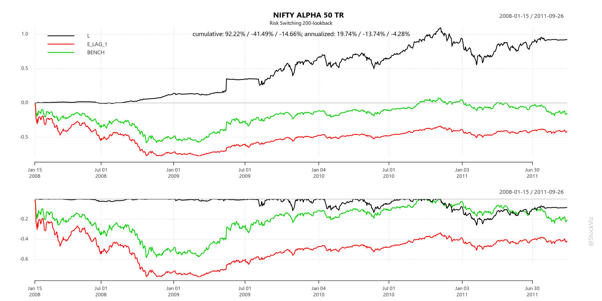
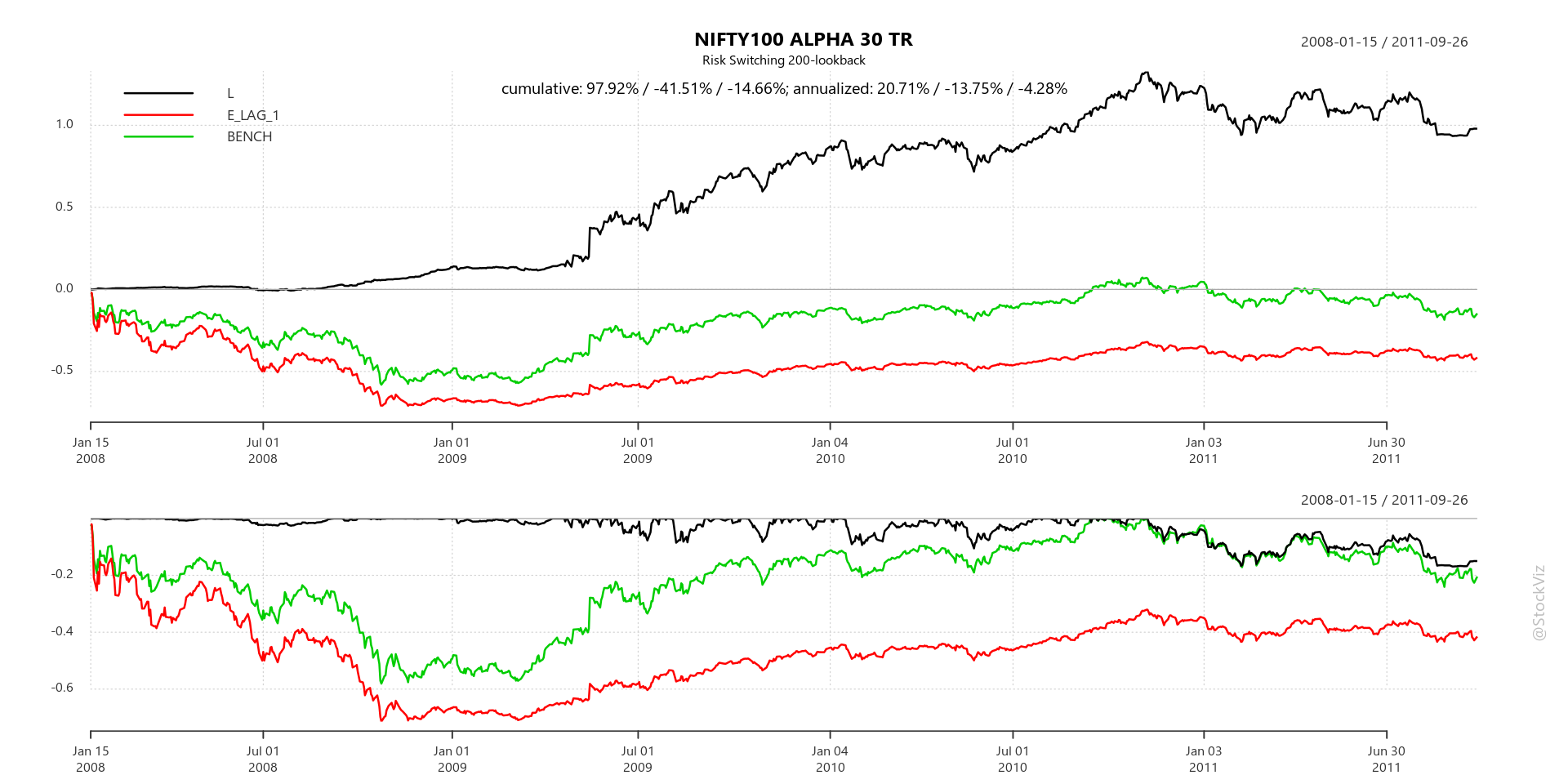
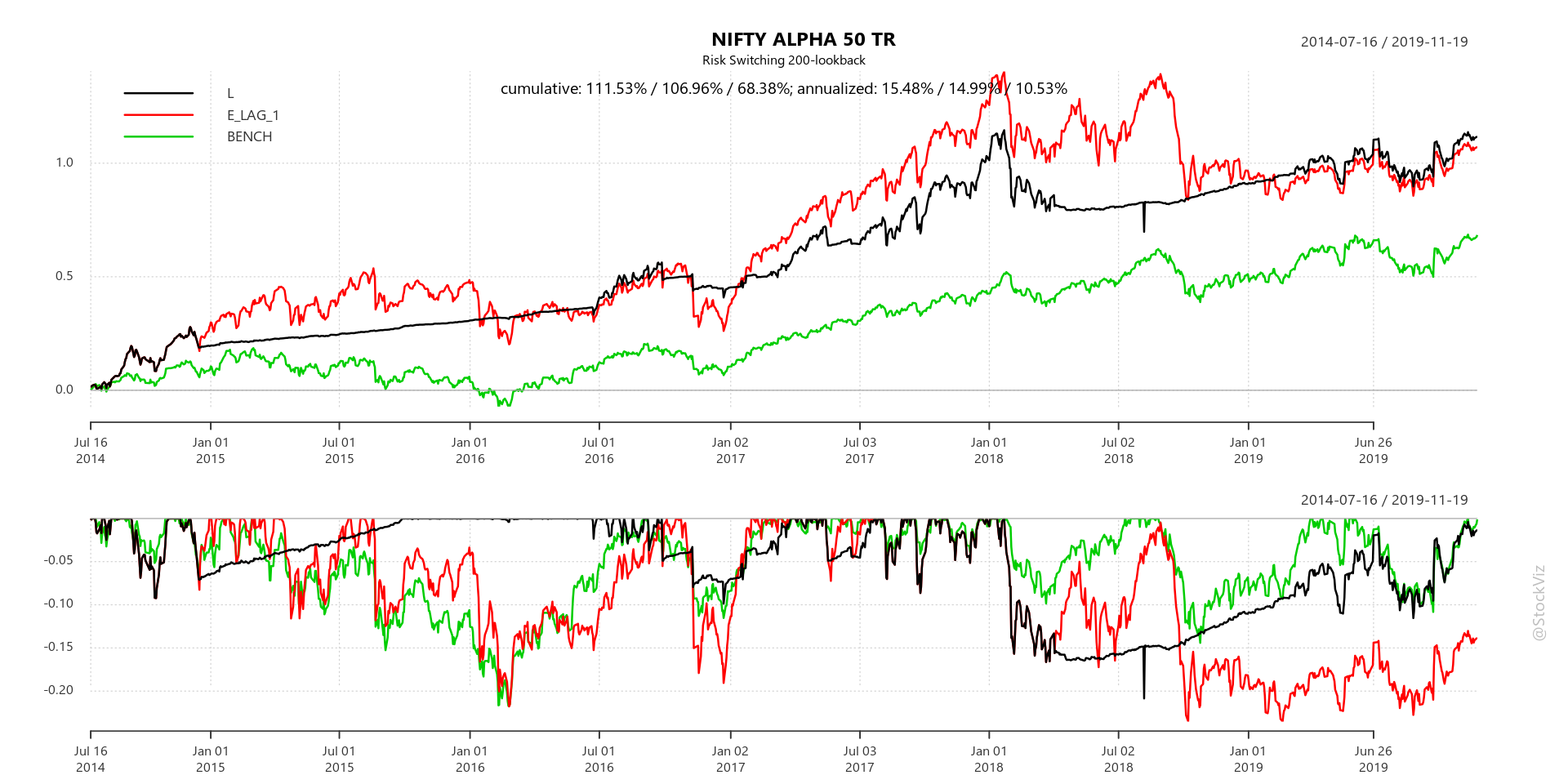
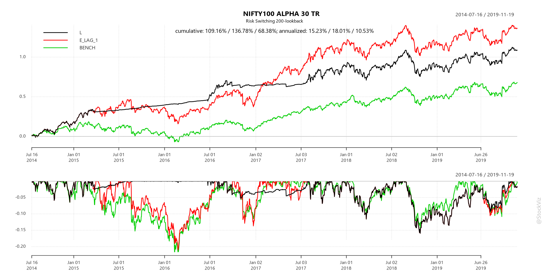
Test Out-of-Sample

Applying a 200-day lookback on both the indices over the test set, we find that the strategy continues to side-step drawdowns but no longer out-performs buy-and-hold by a large margin.

Conclusion

Using historical volatility (std. dev.) reduces drawdown risk in Alpha indices. But it comes at the cost of reduced overall returns over buy-and-hold over certain holding periods. However, given the magnitude of the dodge in 2008 and 2016, it is well worth the effort (and cost) if it helps keep the discipline.

Check out the code for this analysis on pluto. Questions? Slack me!

Categories Investing Insight Tags momentum, NIFTY, volatility

Does Momentum Trend or Mean-Revert?

shyam September 26, 2019September 26, 2019

Outline

We consider long-only momentum returns to be composed of market returns plus excess returns.

If excess returns over a specified period, n-days, (say, 5- or 10-days) either trends or mean-reverts, then that can be used to trade the momentum portfolio.

One way to check if a time-series is trending is to calculate the Hurst exponent (H) over a rolling window (say, 5-years) of n-day excess returns . If H < 0.5, then the time-series is mean-reverting; if H > 0.5, then it is trending, else it is random.

A simple strategy would be, for H < 0.5 (mean-reverting), if excess returns is greater than its median, then exit or if excess returns is less than its median, then enter.

The problem boils down to specifying the excess-return calculation periods (n-days) and the Hurst exponent rolling windows so that it makes sense (avoid data-mining.)

Setup

We use the Barclays Euro-zone, UK, Japan and US momentum index data-sets to run our experiment. Since they provide both an excess-return index and a total-return index, we can use the former to time entries and exits in the latter.

We ran for two n-day configurations: 5 and 10. We set the Hurst (and median) rolling window at 5-years.

We expected to find H to be either consistently above or below 0.5. My personal expectation was that H would be above 0.5 (trend.)

Results

Using the Hurst exponent did not improve momentum returns. In both 5-day and 10-day configurations, a strategy that went long if n-day returns were less than their median out-performed those that incorporated H.

The back-test using 5-day returns mostly worked on Euro-zone and US momentum indices. So we are skeptical that this approach can be generalized and it will likely fall prey to data-mining.

The back-test using 10-day returns saw buy-and-hold emerge a consistent winner.

The 5-day H toggled between trending and mean-reverting but spent most of its time trending. The 10-day H was consistently trending. For the specifications that we tested, momentum excess returns trends.

Code and Charts

The R code is here: 5-day and 10-day config. You can login to pluto and play around with the lookback and statWindow variables to see how H, median and back-test results change.

Questions? Ask them over at our slack workspace.

Categories Investing Insight Tags momentum, quant

Are Stop-Losses Worth It? Part II

shyam May 2, 2019

We saw how, in aggregate, stop-losses do not add any value to a momentum portfolio after taxes and transaction costs (Are Stop-Losses Worth It?) When you dig a little deeper into the actual positions that get stop-lossed and analyze their subsequent returns, we find that, on average, subsequent returns are not negative enough to justify trading costs.

During mid-2016 through April-2019 Bull and Bear phases

Here’s how the Momo (Relative) v1.1 Theme’s stop-lossed positions behaved 20-days after they got booted out, mid-2016 through April-2019:

Summarized statistics across different holding periods:

Now let’s partition the total period into two. The first part covers the “bullish” market of mid-2016 through Dec-2017 and the second Jan-2018 through April-2019.

During the mid-2016 through Dec-2017 Bull

Summarized statistics across different holding periods:

During the Jan-2018 through April-2019 Bear

Summarized statistics across different holding periods:

Conclusion

When looked at from the perspective of a single position, a stop-loss removes red ink and is out-of-sight/out-of-mind. However, it is only when you look at their subsequent returns in the aggregate, that you realize that peace-of-mind comes at a cost.

During the bull phase, when the whole market was shooting higher, stop-lossed positions recovered from their losses. Note how the skew is slightly positive. Stop-losses here were a definite drag after taking costs into account.

During the bear phase, it does look like stop-losses helped – the subsequent returns of stop-lossed positions were skewed left. However, as we saw in our previous post, in aggregate, they did not add value after taking costs into account.

Categories Investing Insight Tags momentum, returns

Are Stop-Losses Worth It?

shyam April 25, 2019

StockViz introduced Themes back in August 2013. We went live with two strategies: Momentum, rebalanced once a month, and Quality to Price, rebalanced once a quarter. The Modi bull market was just getting started and returns were spectacular in the beginning. Here is Momentum, from Jan-2014 through Dec-2015:

And then, in Jan-2016, the Chinese market crash rippled through world financial markets (WaPo). Momentum collapsed. This is the previous chart extended to June-2016:

Momentum investors clamored for a safety net. Enter stop-losses. We created a new set of Themes, called Momos, that had a 5% trailing stop loss at the position level. Positions hitting the stop loss were substituted with stocks that had favorable momentum and trend. The logic was that if the entire market crashed, the strategy would be in cash until stocks gained momentum. We introduced these Themes in June and they worked as advertised on the subsequent market correction in November that year. Idea validated? Here is a chart comparing the returns of Momentum (vanilla) vs. Momo (Relative) v1.1:

Momo trails its plain-vanilla counterpart over a ~3 year period. There has been plenty of volatility during that time – November 2016, August 2017 and January 2018 through now. And Momo traded a lot more than its plain-vanilla counterpart (the turnover charts are on the Theme pages linked above) through these bouts of volatility. And what was saved through stop-losses was paid for in taxes and transaction costs. Here is a chart that shows the Momo strategy with and without transaction costs:

So, are stop-losses worth it? Probably not. It is very difficult to de-risk a high-risk strategy intrinsically. It is better for investors to focus on asset allocation to bring down overall portfolio volatility to a level that they can bear. Think of it like trying to tame a tiger. You may very well succeed. But a tame tiger is a cat.

Categories Investing Insight Tags momentum, returns

Momentum vs. Low Volatility

shyam March 19, 2019

Is the low-volatility anomaly overrated?

Investors may be giving up on the significantly higher returns of a momentum strategy in favor of slightly lower drawdowns of a low-volatility strategy. They maybe better off managing overall portfolio risk through a bond allocation rather than tilting away from momentum.

Categories Investing Insight Tags momentum