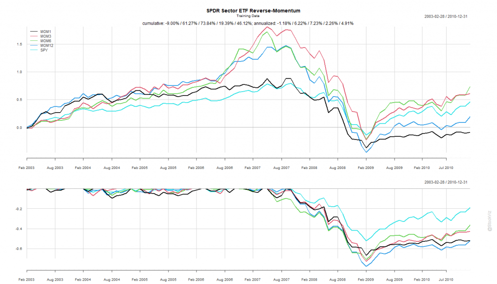
Previously, we saw how buying the best performing sector and holding it for a month didn’t quite pan out. What if, we bought the worst performing sector instead? The “Dogs of Sector Spiders,” if you will.
Calculate rolling returns over n months. Where n = 1, 3, 6, 12.
For the n+1th month, go long the ETF that had the lowest return in Step 1.
Like before, we split the dataset into Before 2010 and After 2011.
Pick your Fighter
The Before 2010 dataset shows rotation by 3- and 6-month look-back periods to be better than buying-and-holding the S&P 500.
The 6-month look-back rotation strategy – MOM6 – would’ve been the strategy to bet on.
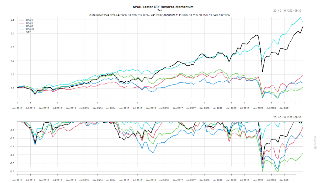
The SPY Rope-a-Dope
“Sure-things” don’t exist in finance.
MOM6 spent the last decade getting absolutely decimated by the S&P 500.
Once again, by simply holding onto the ropes, a passive buy-and-hold S&P 500 investor would’ve come out miles ahead of someone who employed this rotation strategy.
While introducing S&P 500 sector ETFs, we showed how the cross-correlations between them were unstable. This makes developing simple strategies challenging. One common momentum strategy is to simply go long whatever worked best in the previous period.
Rules of Rotation
For ETFs: XLY, XLP, XLE, XLF, XLV, XLI, XLB, XLK, XLU, and SPY
Calculate rolling returns over n months. Where n = 1, 3, 6, 12.
For the n+1th month, go long the ETF that had the highest return in Step 1.
In Step 2, if the selected ETF has -ve returns, stay in cash and earn zero.
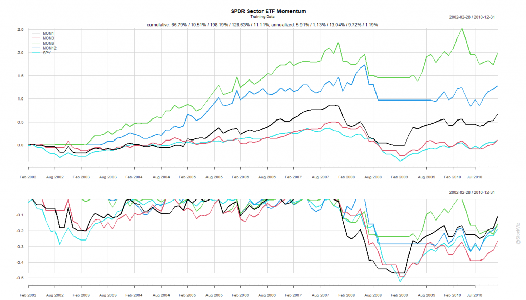
We split the dataset into Before 2010 and After 2011.
Pick your Fighter
The Before 2010 dataset shows rotation by all look-back periods to be better than buying-and-holding the S&P 500.
Probably because of the prolonged dislocation caused by the GFC in 2008 and 2009, all rotation strategies based on the rules above exhibited great stats.
The 6-month look-back rotation strategy – MOM6 – gave an annualized return of 13.04% vs. S&P 500’s 1.19%. Coming out of the crisis, this would have been the fighter to bet on.
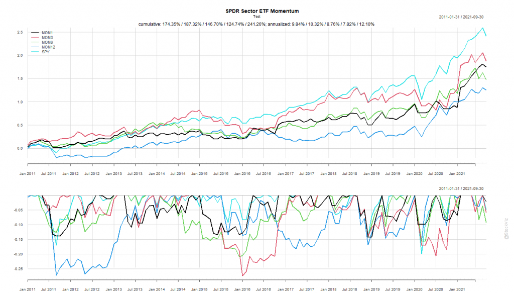
The SPY Rope-a-Dope
In boxing parlance, a “Rope-a-Dope” is
When you maintain a defensive posture on the ropes in an attempt to outlast or tire your opponent. It is most recognized and was actually given that name by Muhammad Ali when he employed the technique to defeat George Foreman.
The After 2011 dataset is a prime exhibit of why “sure-things” don’t exist in finance.
The S&P 500 spent the next decade demolishing everything.
MOM6, the winner from our first round, went on to underperform the S&P 500 for the next 10 years by ~4%
By simply holding onto the ropes, a passive buy-and-hold S&P 500 investor would’ve come out miles ahead of someone who employed this rotation strategy.
Momentum investing strategies have historically produced high returns in Indian equities. The biggest problem with them has been deep drawdowns when the markets enter bear territory.
A number of risk management strategies like using moving averages, trailing stop-losses, and hedging have been discussed on this blog before. These strategies, either standalone or in combination with each other, have provided investors with significant protection against momentum crashes. These are “exogenous” techniques, i.e. they are not part of the strategy itself but is imposed by portfolio management infrastructure. The advantage of these techniques is that the default is to be always invested in the market. It is risk-management’s job to control exposure.
Alternatively, endogenous risk-management techniques are those that are baked into the investment strategy itself. Our All Star strategy is a prime example of a momentum strategy that reduces exposure to equities by design. If enough stocks are not hitting their all-time-highs, it simply sits in cash. When you combine this with one of the exogenous risk-management techniques, you end up with a high Sharpe portfolio.
The advantage of high Sharpe strategies is that you can use leverage to amplify returns. However, if you are a “cash-and-carry” investor then it might be too conservative. Is there a momentum strategy that sits between All Star and traditional momentum?
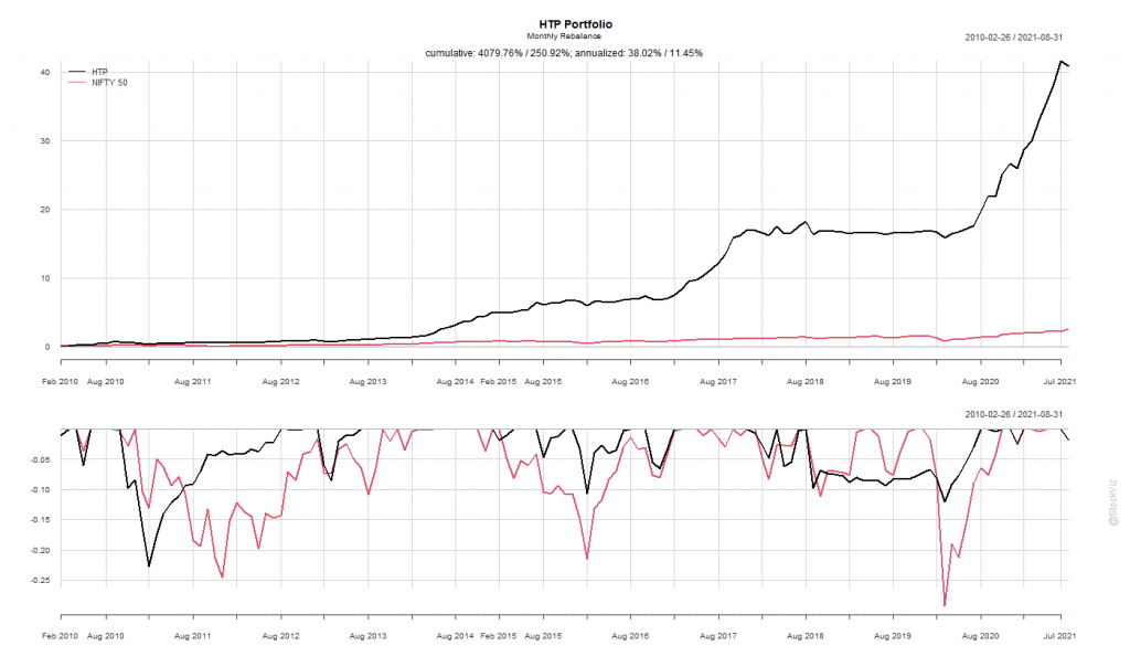
High-to-Price (HTP) Momentum
A new paper, Büsing, Pascal and Mohrschladt, Hannes and Siedhoff, Susanne, Decomposing Momentum: Eliminating its Crash Component (SSRN,) outlines a new way to slice the 52-week momentum strategy to avoid crash risk. It describes a ranking system based on High-to-Price (HTP) where HTP = ln(Phigh/P0) where Phigh is the stock’s 52-week high price and P0 is its price at the beginning of the period.
A monthly rebalanced HTP long-only portfolio looks promising. It sidestepped quite a few whipsaws and has a better drawdown profile than NIFTY 50.
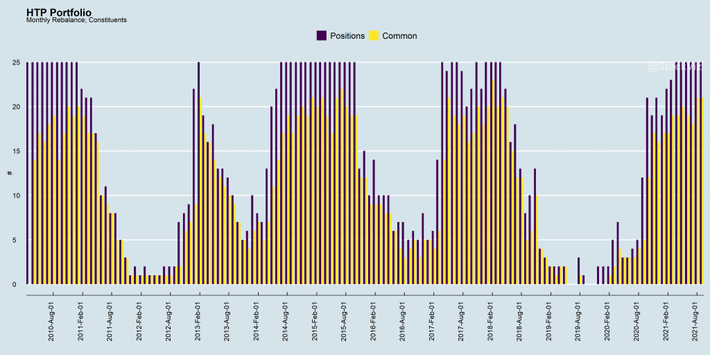
There have been periods where the strategy couldn’t find 25 stocks to go long and it only had a handful of positions or was all cash. However, the degree of overlap between constituents in consequent months is quite high indicating that the portfolio is likely to experience very low churn. In this aspect, it is very similar to the All Stars strategy.
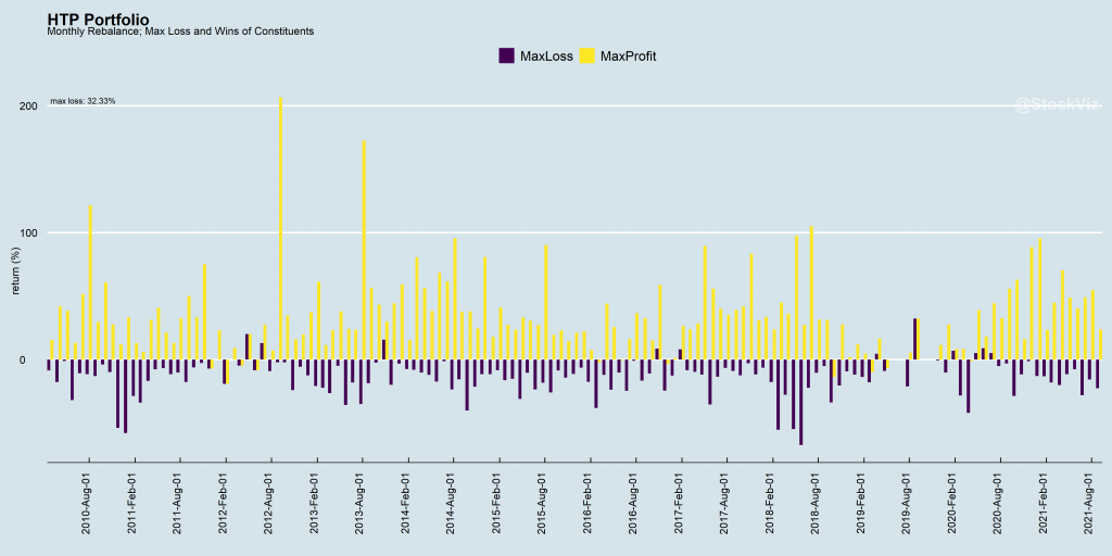
At a line-item level, there have been instances where some stocks have tanked more than 30% in the month. However, the skew is, by-and-large, positive.
Investing in HTP Momentum
The real world doesn’t line-up perfectly to match the end-of-the-month rebalancing activity outlined in our backtest. To make this strategy investible, it needs to have some risk-management strategy in place on a clearly defined universe of stocks and has to be dynamically rebalanced.
We present our High-to-Price (HTP) Momentum Theme that consists of a portfolio of 25 stocks selected from the top 300 stocks by market-cap that rank high on their HTP scores. A 10% trailing stop-loss ensures that errant positions don’t drag down the whole portfolio. It is ideal for investors who can accept a bit more risk than All Stars for potentially higher returns.
Factor performance tends to be sticky. If Value, Momentum, Quality, etc. out-performed in the recent past, they continue to out-perform in the near-future.
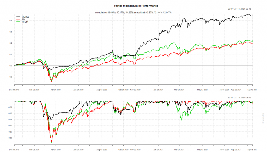
The performance of the US portfolio has been gangbusters. It sidestepped the Corona Crash of 2020 and has been on a tear since then. The Indian experience, however, has been disappointing.
US Factor Momentum
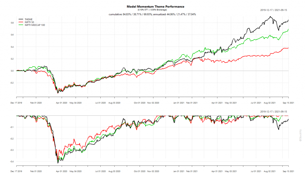
The Indian portfolio suffered from its inability to go into cash/bonds during crashes. Being fully invested took a bite out of its overall performance.
India Factor Momentum
The Indian version comes up short even if you compare its stats with its component factor portfolios.
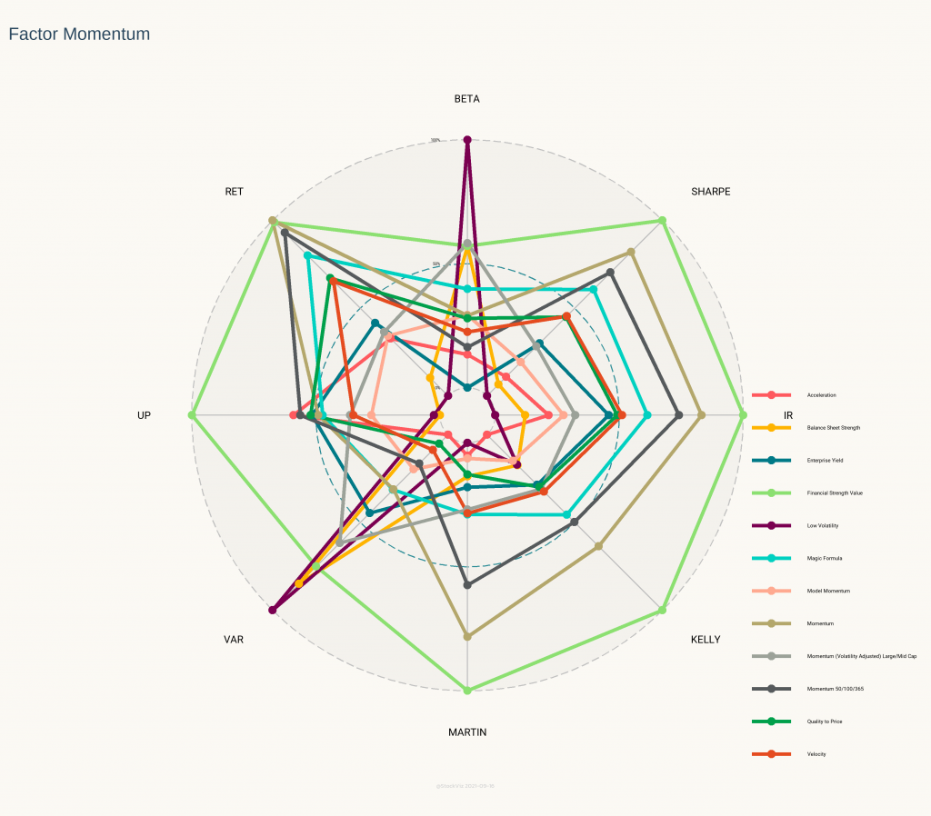
India Factor Momentum Statistics
The intuition behind the Radar Plot above is that the larger the area under the points, better the strategy. Model Momentum is in pink and it pales in comparison to most of its constituents. Surprisingly, the Financial Strength Value Theme (light green,) that is rebalanced annually, beat out everything else.
What explains the underperformance?
Not being able to go into cash/bonds meant a larger hill to climb during recoveries. However, cash is a double-edged sword. If you get the timing wrong, you might end up going into cash after the bottom and watch the market recover helplessly. Unless the trend formation period is really short, cash is not a viable option.
High transaction costs can also be playing a role here. The difference between Gross and Net returns is ~15%. Not as high as a pure momentum strategy but not trivial either. Also, US portfolios do not incur STT and brokerages are essentially zero.
Maybe 20-months is too short a window to judge such a slow-moving strategy. The research looks solid and maybe all we need is to give it some time?
Gary Antonacci created the Global Equities Momentum (GEM) model that applied dual momentum to stock and bond indices. It toggles between stocks and bonds using 12-month trailing returns. And when it toggles to “stocks,” it chooses between US equities and International (ex-US) equities based on whichever posted higher returns in the previous 12-months. The model uses the S&P 500 index as a stand-in for US equities and the WORLD ex USA index for international stocks.
Investors can use the ETFs SPY/VOO for the S&P 500, SCHF for World ex-US DMs and AGG for bonds while replicating this strategy.
The best part about this strategy is its simplicity. It takes just 3 inputs and anybody can set it up on Google Sheets. Execution is as simple as it gets because at any given point in time, it is long just one ETF. Also, given that it uses a 12-month look-back, it is less prone to whiplashes, resulting in a lower trading frequency.
Specifications & Expressions
When you automate systematic strategies, you need to nail down its exact specifications. In this case, they are mainly: inputs, look-back periods and traded instruments.
The original version of the Strategy uses the S&P 500 and World ex-US both for inputs and as proxies for the traded instruments. However, there is no reason why they both should be the same. Also, what is so magical about a 12-month look-back period anyway? Why can’t it be 6 -months, a month or an average of the last 6-months?
The Strategy only describes a broad idea with one set of Specifications and Expressions out of a multitude. It can (and should) be adapted to fit one’s risk profile and investment horizon.
The Momentum Expression
The easiest tweak to the original strategy is to swap out the traded equity instruments with their momentum counterparts.
At the final step, when it comes to executing the trade, you can use MTUM, the US Momentum ETF instead of SPY/VOO and IMTM, the DM ex-US Momentum ETF instead of SCHF.
Long-only momentum ETFs are highly correlated to their market-cap counterparts but have the potential to juice returns in bull-markets. Since we are trend-following anyway, why not go a step further up the risk-curve and embrace momentum as well?
Picking a look-back for trend-following strategies is fraught with data-mining bias. One could potentially test 100s of periods and pick one that gave the best results historically. The data-mined look-back could even work in forward tests but inexplicably, and suddenly, fail in real portfolios.
The safest thing to do would be to not change the look-back periods outlined in the original research. However, the world would’ve changed since its first publication. How do you strike a balance between the two?
Long look-backs are slow at reacting to rapidly changing markets. Some might say that this is a bug while some might argue that this is a feature. Shorter look-backs, on the the other hand, can react faster but are prone to head-fakes and whiplashes.
The second version of our GEM strategy tries walk the fine line by taking the average of 6- through 12-month returns. It tries to hew close to the original research while acknowledging that the world has gotten faster since it was first published.
No Free Lunch
While the strategy adapts to the broad, slow-moving macro theme of US equity under-performance vis-à-vis rest-of-the-world (were it to occur,) it is not immune to getting whiplashed due to short and steep market dislocations like the COVID crash of March 2020. The strategy got into bonds just when the equity markets were recovering and stayed there until well-after. It is simply not possible to avoid all landmines when it comes to investing.
While we ran our back-tests, we tried a fair amount of permutations and combinations. Some where discarded in spite of having better risk-adjusted returns because they lacked internal consistency. While some slipped into data-mining territory in spite of our best efforts to avoid it. Readers interested in the process and the code can read through our GEM Collection.