Previously, we discussed how removing information from data can be useful. And our discussion on using Euclidean Distance for Pattern Matching showed how you can use a rolling window to identify matching segments within a time-series. What if we mix the two ideas together?
If you transform a time-series of returns to 0-1, then we can use Hamming distance, a measure the minimum number of substitutions required to change one string into the other (Wikipedia,) as a measure of similarity.
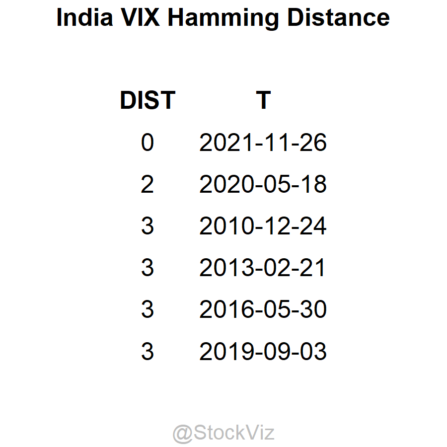
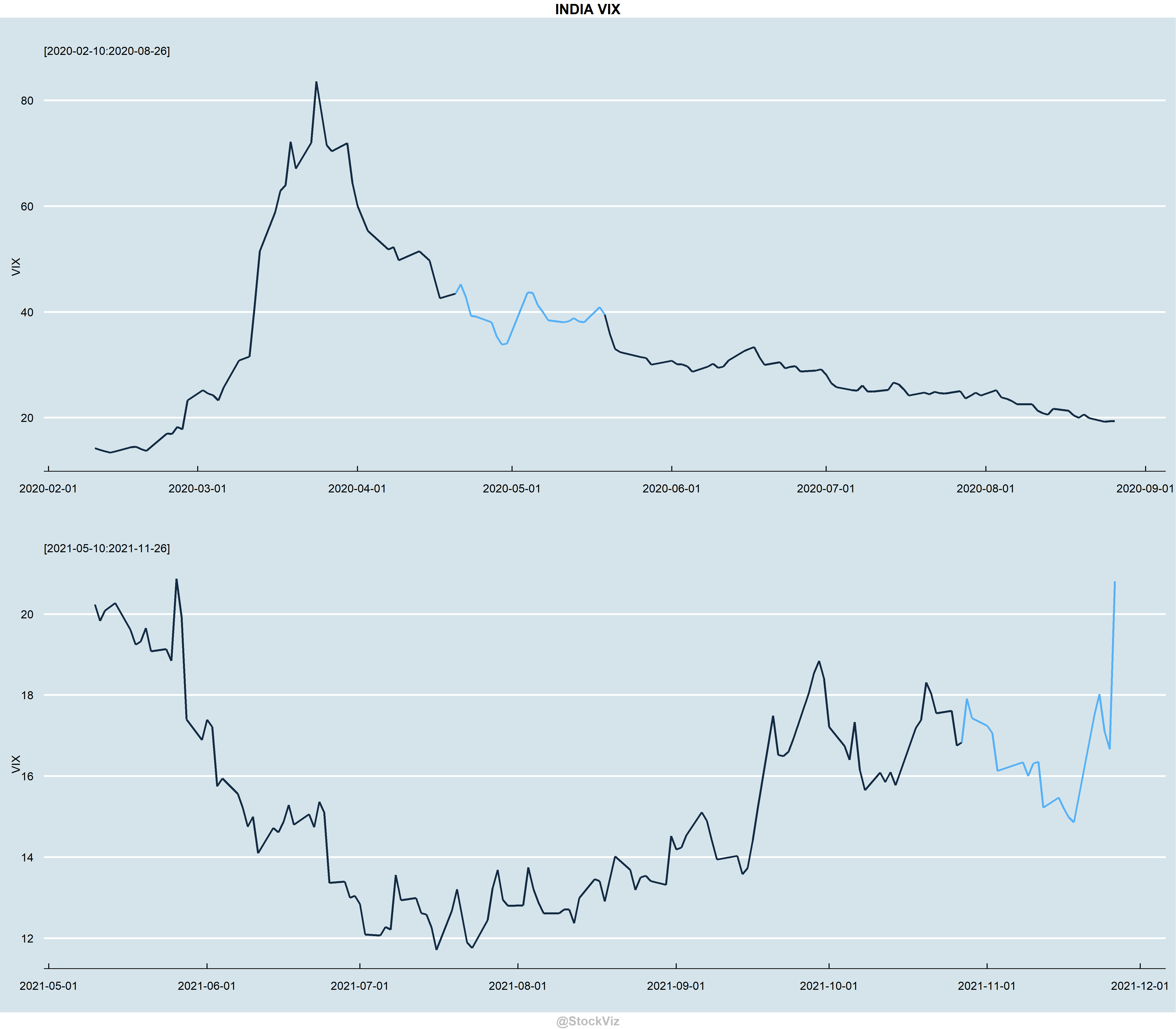
For example, take the most recent 20-day VIX time-series and “match” it with a rolling window of historical 20-day VIX segments and sort it by its Hamming Distance.
Here, on the second row, we see that by just flipping two bits, the 20-day sequence ending on 2020-05-18 matches with the 20-day sequence ending 2021-11-16.If you are looking for a rough up/down days match, then this is a blistering fast way to compute it.
Sometimes, it is useful to remove information from the data that you have.
Lets say, you have a time-series of returns: +0.001, +0.001, +0.001, +0.1, -0.01, -0.01. What if, you removed magnitude information and kept only the direction? You end up with: UP, UP, UP, UP, DN, DN. Now, you can analyze this transformed dataset using a whole bunch of algorithms designed to work on binary sequences.
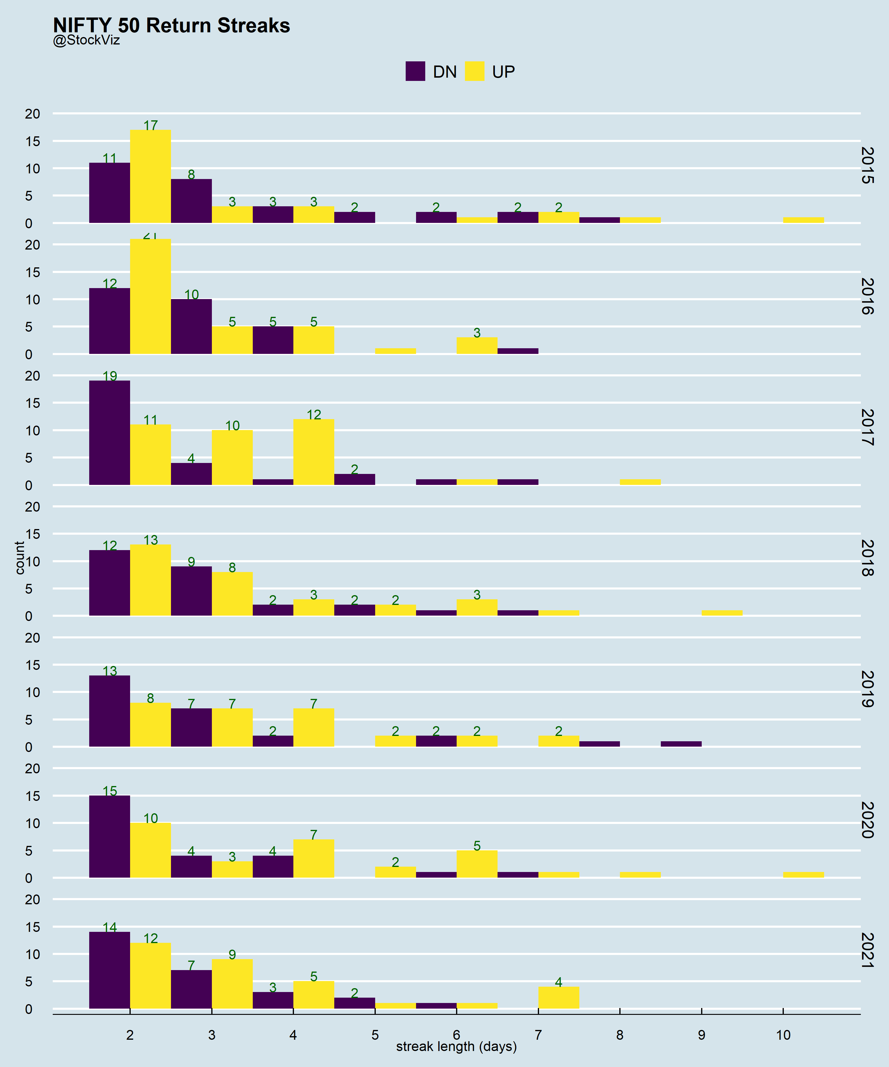
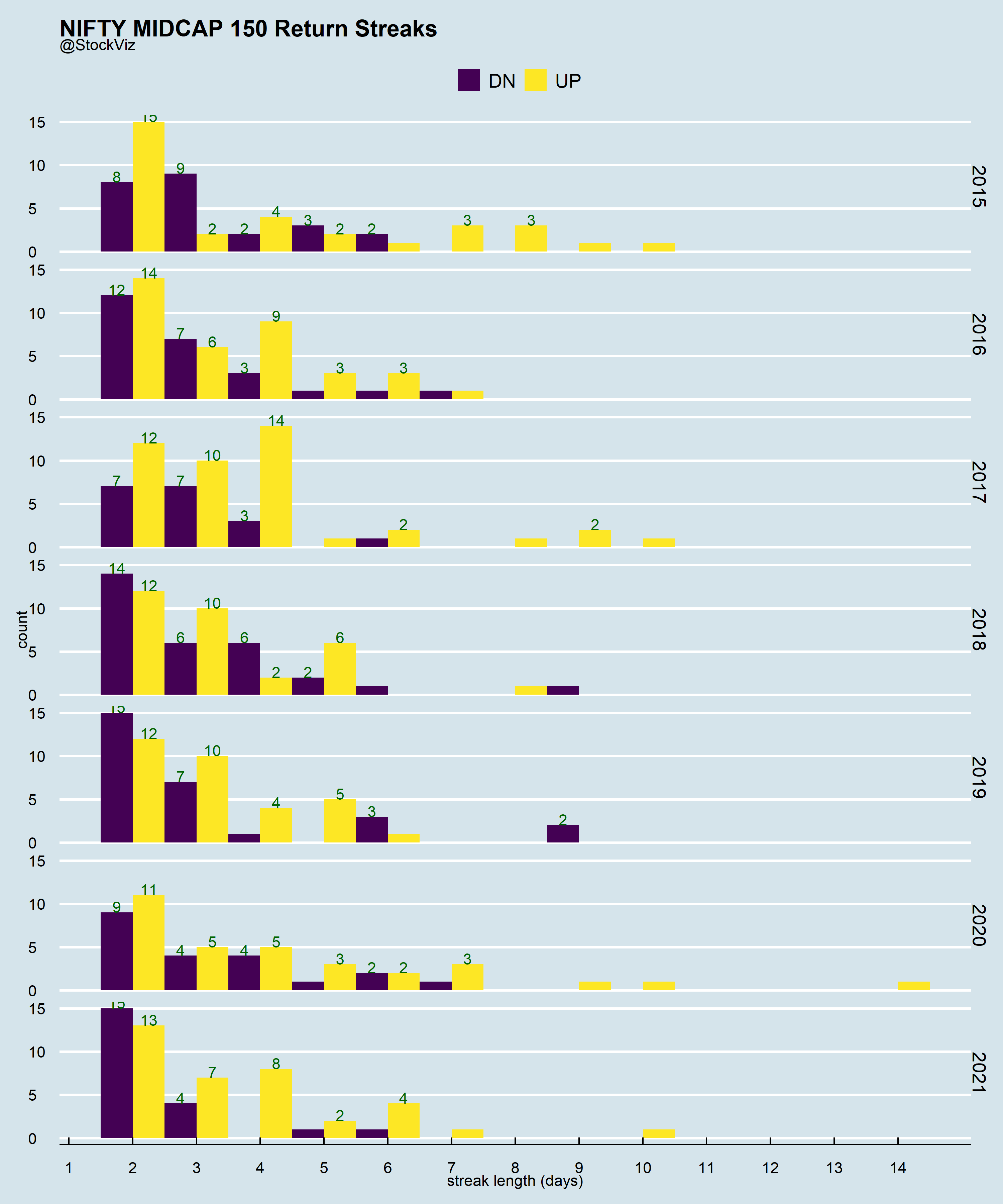
Run Length Encoding (rle) is one such algo. We used it while looking for streaks (Part I, Part II.) We dismissed the backtest as a datamining artefact. Which it might very well be. However, if you believe that a timeseries can exhibit both trend and mean-reversion, then looking at it through this lens can be useful.
Knowing the “average” length of streaks can also help in position sizing in a trend-following system and regime classification.
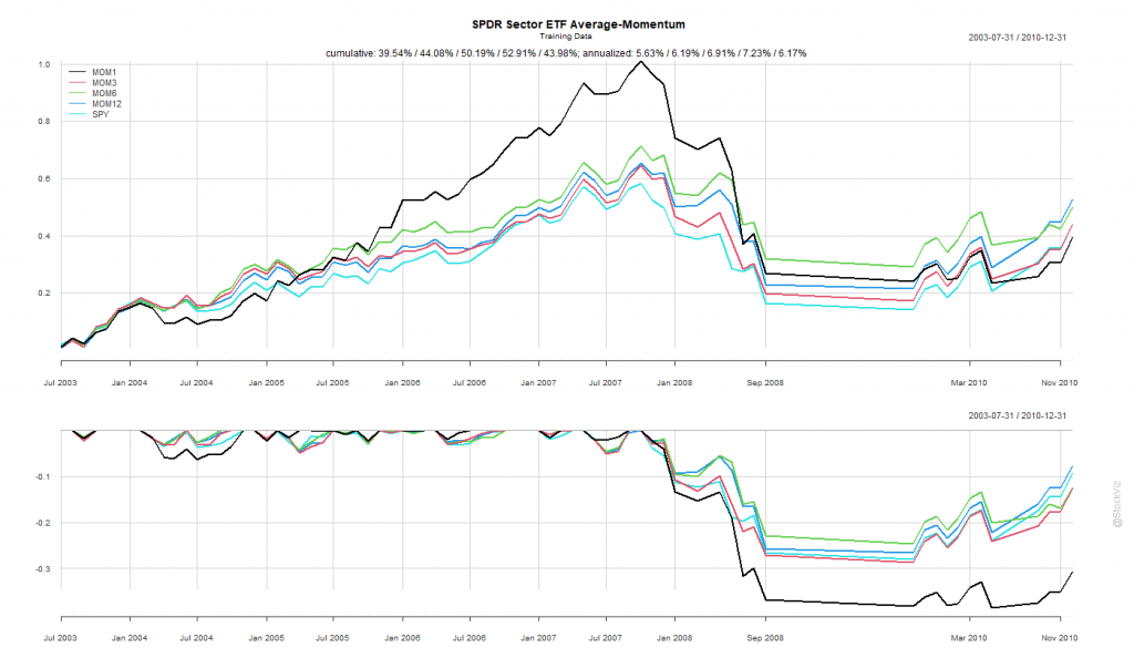
We’ve been having a bit of fun with the S&P Sector “Spider” ETFs: Intro, Momentum, Anti-Momentum. We saw how strategies that backtested well with pre-2011 data failed later. In this post, we see if buying all ETFs with a positive return over n-months help us beat the S&P 500 index.
Calculate rolling returns over n months. Where n = 1, 3, 6, 12.
For the n+1th month, go long the ETFs that had positive returns in Step 1.
Like before, we split the dataset into Before 2010 and After 2011.
Pick your Fighter
The Before 2010 dataset shows rotation by 6- and 12-month look-back periods to be better than buying-and-holding the S&P 500.
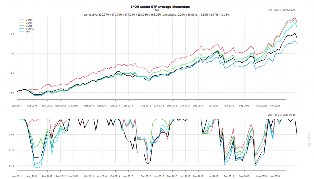
The SPY Rope-a-Dope
MOM6 and MOM12 were too close to call in the training set. If you had “course-corrected” after the first couple of years of under-performance of MOM12 and switched to MOM6, you would’ve out-performed. On the other hand, staying the course would’ve meant losing out to the mighty S&P 500.
Once again, by simply holding onto the ropes, a passive buy-and-hold S&P 500 investor would’ve come out miles ahead of someone who tried to time sectors systematically.
What did we learn?
We tested a few basic allocation strategies that investors typically use to approach the “rotation” problem. Some of them worked well in the training set but their performance failed to carry over. Besides, if you add transaction costs and taxes, we are not sure if it was worth the effort given the post-2011 market regime.
Maybe there are more sophisticated qualitative/fundamental ways to approach this problem that work. However, most media articles about “sector rotation” are written with perfect hindsight and it is near impossible to do it with simple strategies that are accessible to the average investor.
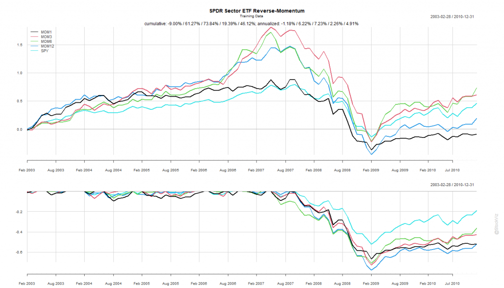
Previously, we saw how buying the best performing sector and holding it for a month didn’t quite pan out. What if, we bought the worst performing sector instead? The “Dogs of Sector Spiders,” if you will.
Calculate rolling returns over n months. Where n = 1, 3, 6, 12.
For the n+1th month, go long the ETF that had the lowest return in Step 1.
Like before, we split the dataset into Before 2010 and After 2011.
Pick your Fighter
The Before 2010 dataset shows rotation by 3- and 6-month look-back periods to be better than buying-and-holding the S&P 500.
The 6-month look-back rotation strategy – MOM6 – would’ve been the strategy to bet on.
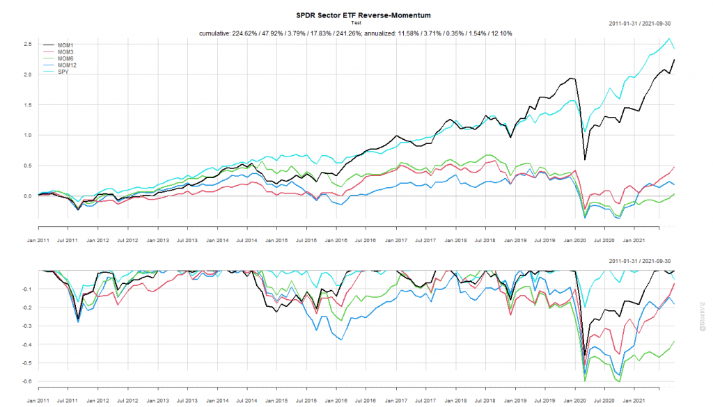
The SPY Rope-a-Dope
“Sure-things” don’t exist in finance.
MOM6 spent the last decade getting absolutely decimated by the S&P 500.
Once again, by simply holding onto the ropes, a passive buy-and-hold S&P 500 investor would’ve come out miles ahead of someone who employed this rotation strategy.
While introducing S&P 500 sector ETFs, we showed how the cross-correlations between them were unstable. This makes developing simple strategies challenging. One common momentum strategy is to simply go long whatever worked best in the previous period.
Rules of Rotation
For ETFs: XLY, XLP, XLE, XLF, XLV, XLI, XLB, XLK, XLU, and SPY
Calculate rolling returns over n months. Where n = 1, 3, 6, 12.
For the n+1th month, go long the ETF that had the highest return in Step 1.
In Step 2, if the selected ETF has -ve returns, stay in cash and earn zero.
We split the dataset into Before 2010 and After 2011.
Pick your Fighter
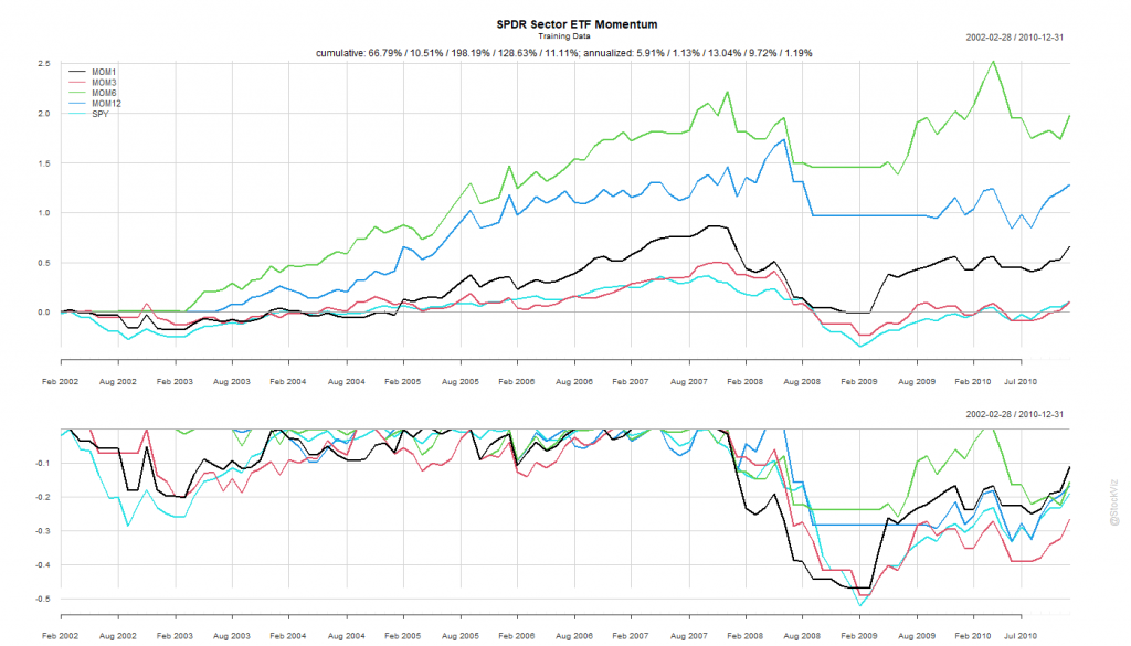
The Before 2010 dataset shows rotation by all look-back periods to be better than buying-and-holding the S&P 500.
Probably because of the prolonged dislocation caused by the GFC in 2008 and 2009, all rotation strategies based on the rules above exhibited great stats.
The 6-month look-back rotation strategy – MOM6 – gave an annualized return of 13.04% vs. S&P 500’s 1.19%. Coming out of the crisis, this would have been the fighter to bet on.
The SPY Rope-a-Dope
In boxing parlance, a “Rope-a-Dope” is
When you maintain a defensive posture on the ropes in an attempt to outlast or tire your opponent. It is most recognized and was actually given that name by Muhammad Ali when he employed the technique to defeat George Foreman.
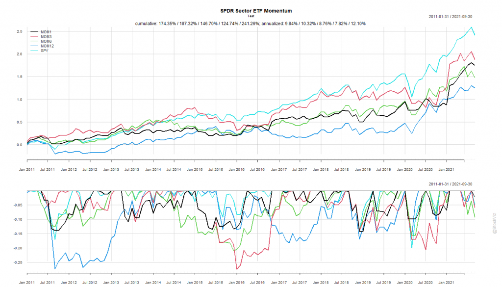
The After 2011 dataset is a prime exhibit of why “sure-things” don’t exist in finance.
The S&P 500 spent the next decade demolishing everything.
MOM6, the winner from our first round, went on to underperform the S&P 500 for the next 10 years by ~4%
By simply holding onto the ropes, a passive buy-and-hold S&P 500 investor would’ve come out miles ahead of someone who employed this rotation strategy.