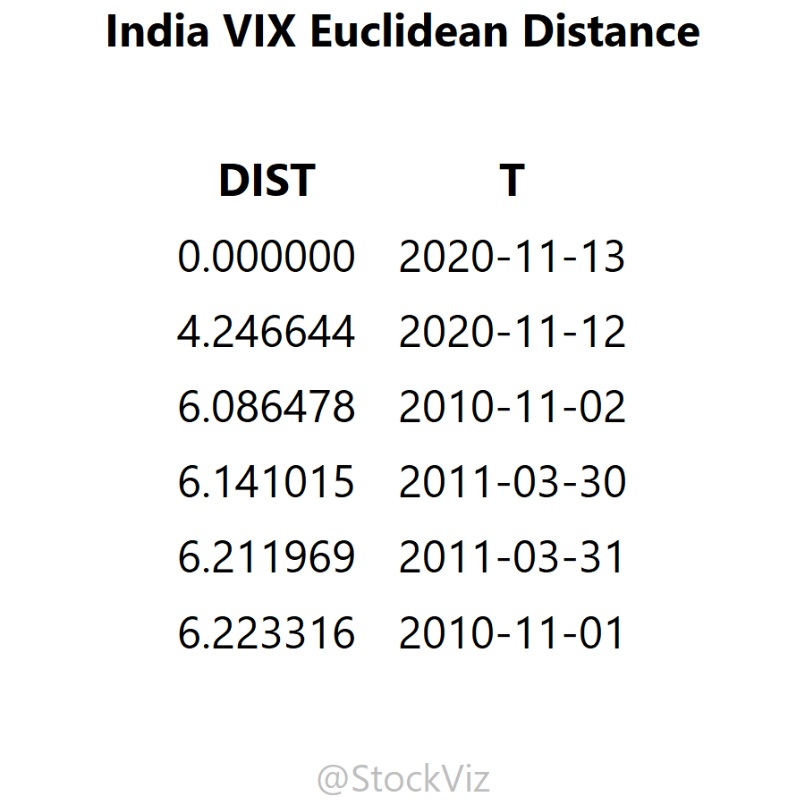
Most of us have learnt how to calculate the distance between 2 points on a plane in high school. The simplest one is called the Euclidean Distance – a pretty basic application of the Pythagorean Theorem. The concept can be extended to calculate the distance between to vectors. This is where it gets interesting.
Suppose you want to match a price series with another, ranking a rolling window by its Euclidean Distance is the fastest and simplest way of pattern matching.
For example, take the most recent 20-day VIX time-series and “match” it with a rolling window of historical 20-day VIX segments and sort it by its Euclidean Distance (ED.)
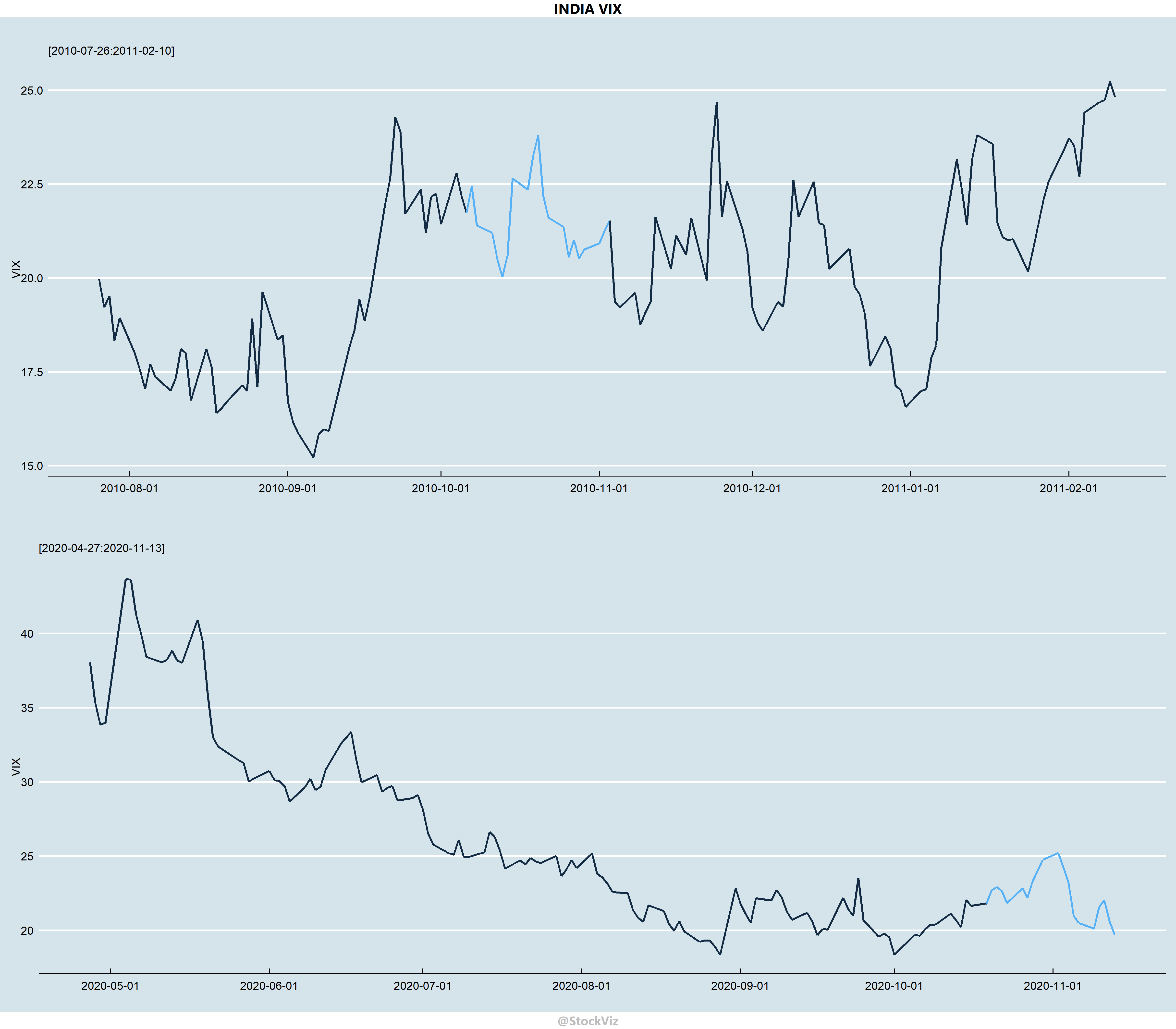
Here, the ED has dug up a segment from November-2010 as one of the top 5 matches. Take a closer look:
While not a perfect match, it “sort of” comes close.
Sometimes, a simple tool is good enough to get you 80% of the way. This is one of them.
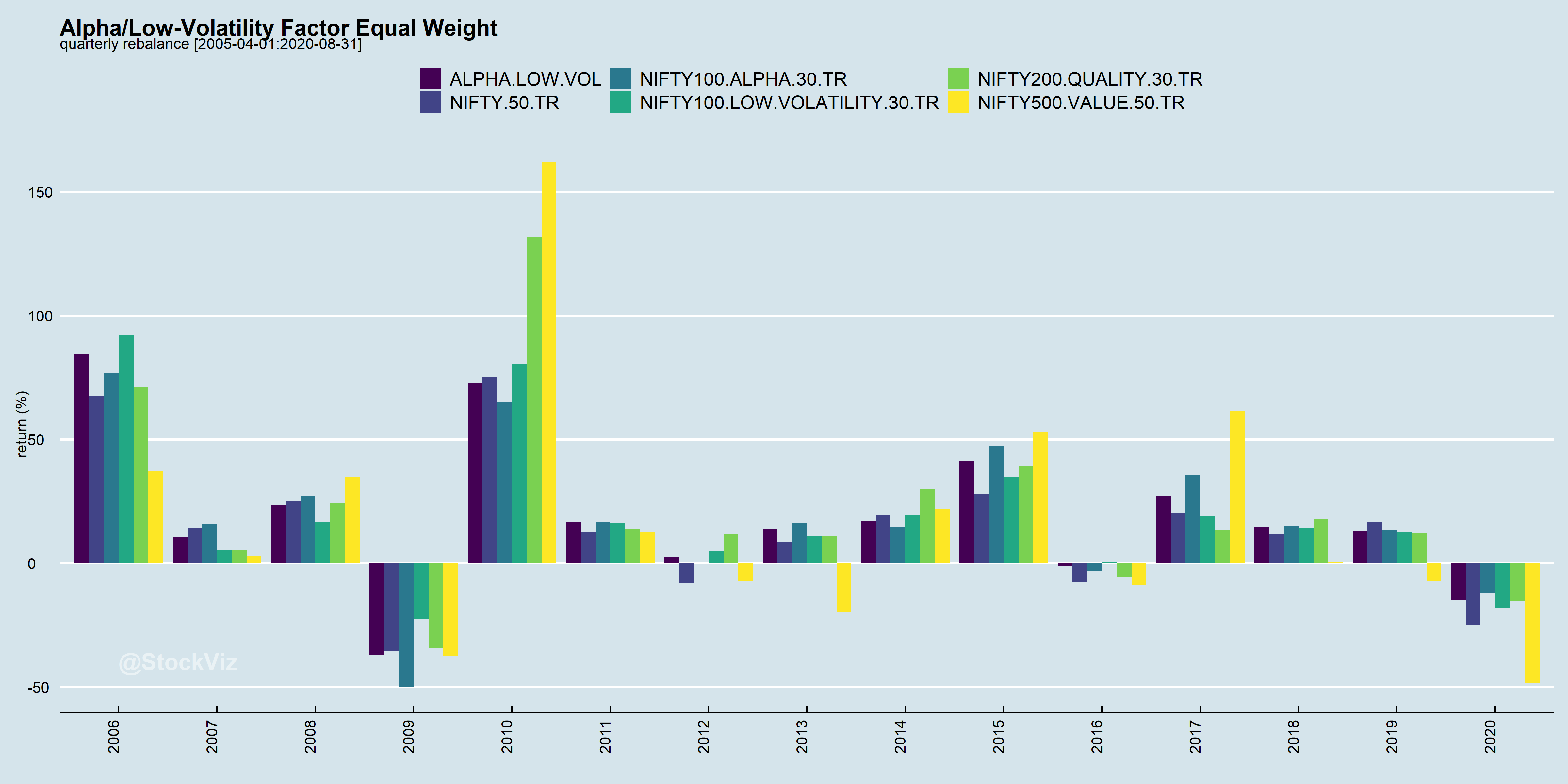
Can’t decide between quality, low-volatility, high-alpha? Why not buy all of them?
Our previous post discussed how you can use the historical performance of different factors to avoid falling into a factor-trap. However, can factor investing be further simplified?
The NSE Strategy Indices
The NSE has published a whole library of factor indices. Some of them are pure factors – like quality, low-volatility, etc – and some are hybrids – like alpha-quality-low-volatility (sort of like a shampoo-conditioner-face-wash 3-in-1.) You can explore their website if your curious.
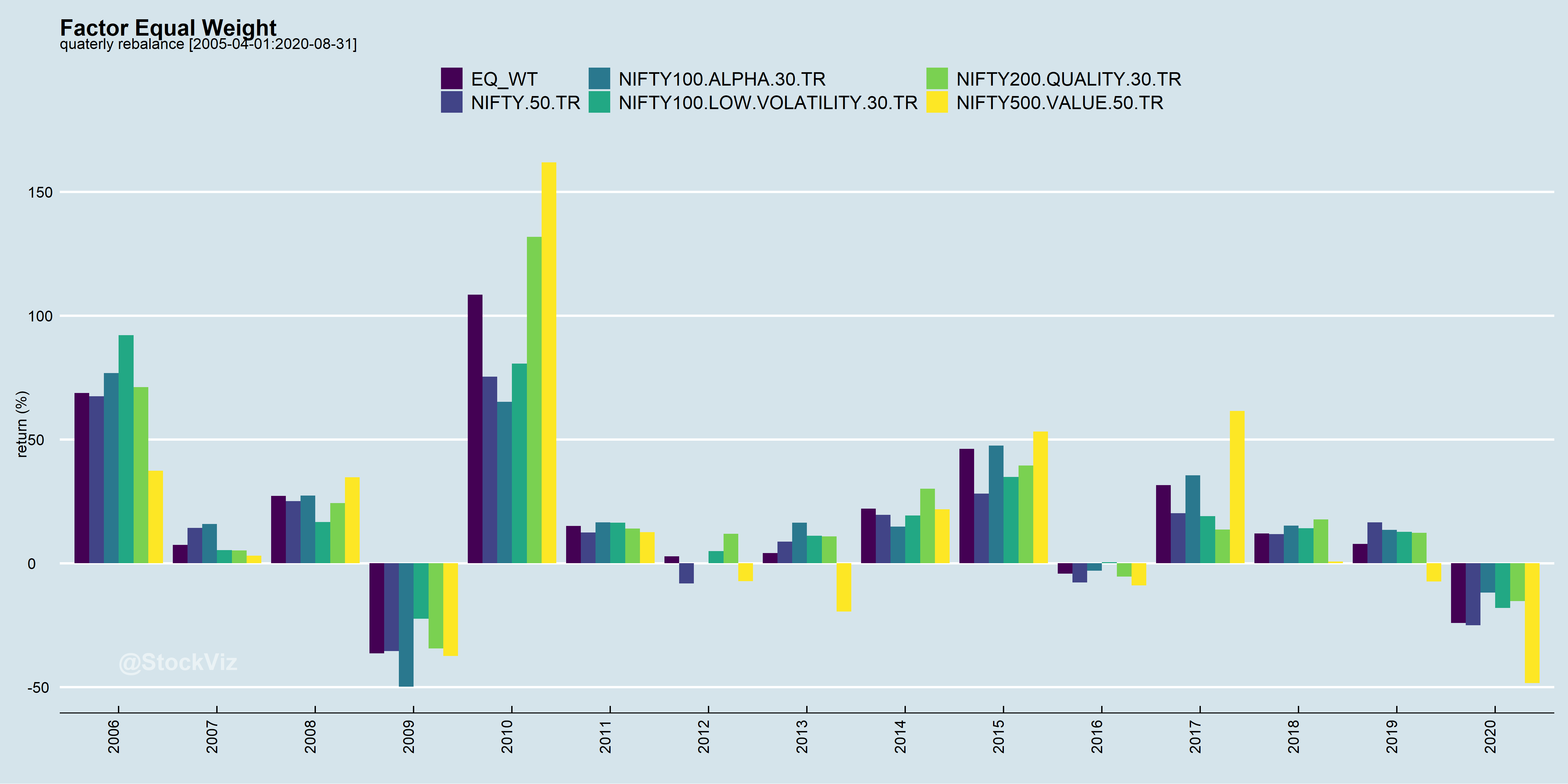
The question is, what if you just took quality, low-volatility and high-alpha (a proxy for momentum) and just equal weighted it? Why choose when you can have all? This is the essence of the Multi-Factor approach to factor investing.
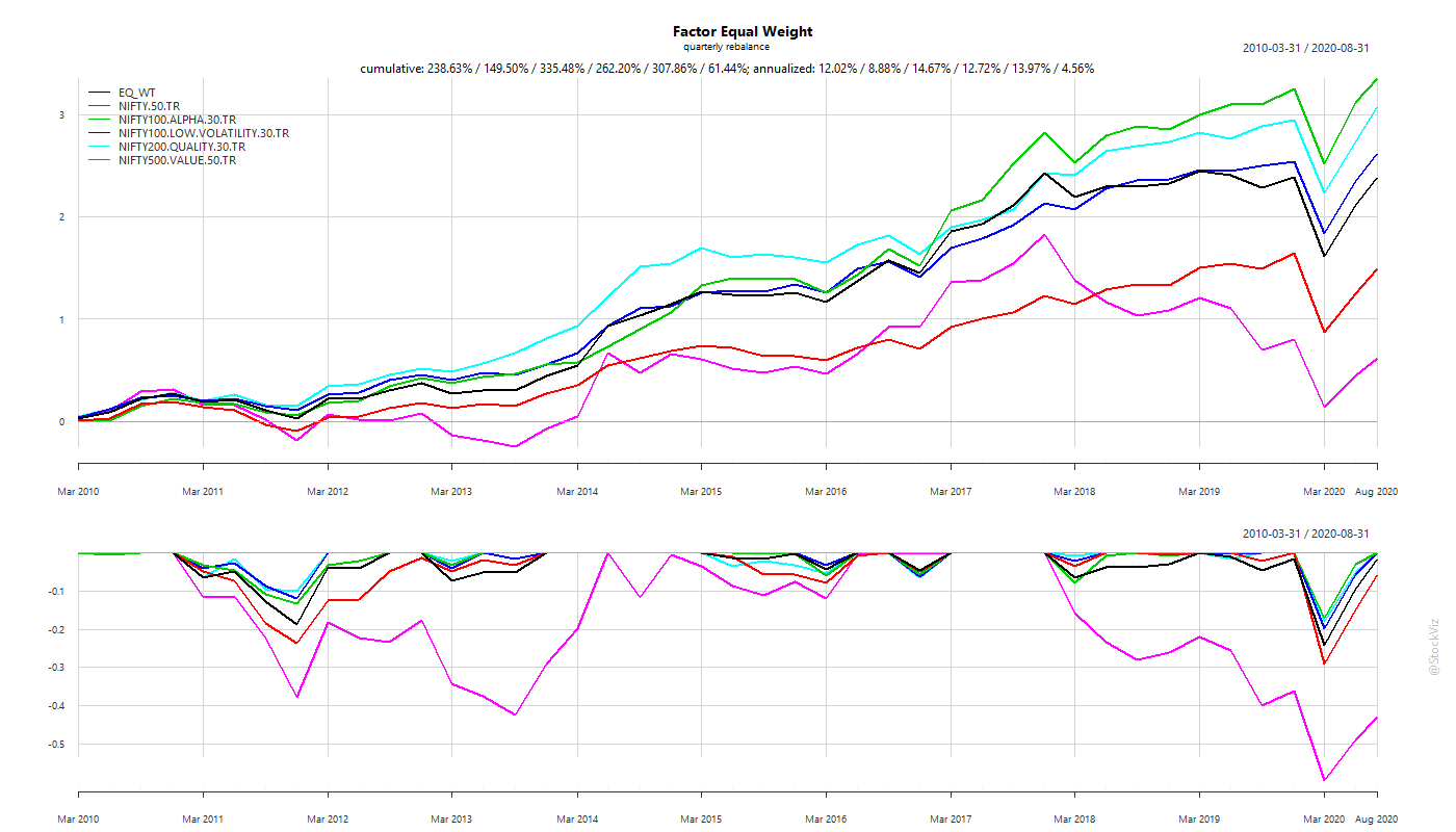
Equal-weighted Factor Portfolio
Even if you did a quarterly rebalance, you did better than NIFTY 50.
Since 2010, an equal-weight alpha/low-vol/quality/value factor portfolio gave an annualized return of 12% vs. NIFTY 50’s 8.88%.
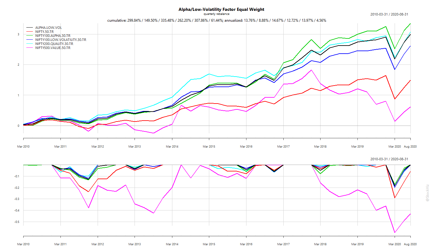
While alpha and low-vol are price-based factors, quality and value are based on company fundamentals. What if, we just equal weighted the price-based factors?
Equal-weighted Alpha and Low-Volatility Factor Portfolio
Given the out-performance of the low-volatility factor, we see a significant boost to an equal weighted alpha/low-vol portfolio compared to equal weighting all the factors.
To summarize returns since 2010,
equal-weight all factors: 12.02%
equal-weight only alpha and low-vol: 13.76%
NIFTY 50: 8.88%
Caveats
Before transaction costs, we see that factor indices have beaten the NIFTY 50, historically. However, investors should bear these points in mind while looking at index back-tests:
Index Inception – the date from which the index was constructed (since 2005.)
Launch – the date on which the index was launched (in 2018.)
Invested – the date from which a significant amount of money gets invested in the index (in 2019.)
Re-balance frequency – how often does the index rebalance?
At launch, these indices have incorporated over 13 years of historical data. One can’t discount the possibility that there might be some over-fitting to increase their marketability.
Typically, index performance dips once the AUM crosses a tipping point. And given that India has a 0.1% STT (Securities Transaction Tax,) the higher the re-balance frequency, the worse the performance.
The true test of these indices will occur when real money is invested in them over two or three complete cycles.
Conclusion
Both Factor Rotation and Multi-Factor approaches have their pros and cons. However, the one thing that remains common is that these take time to play-out. There are huge year-over-year variances in performance and investors need to stick to an approach long enough for alpha to emerge.
Factor investing is the process of constructing portfolios of stocks by isolating certain statistical properties that have shown to out-perform over the long term. For example, investing in stocks that rank high in the “Quality” factor. Here are some factors that were discussed previously on FreeFloat:
While factor portfolios are expected to out-perform over the long-term (say, 30 years,) there is a strong chance that they under-perform over an individual’s holding period (5-10 years.) This leads to sub-par investment returns due to out-of-favor factors.
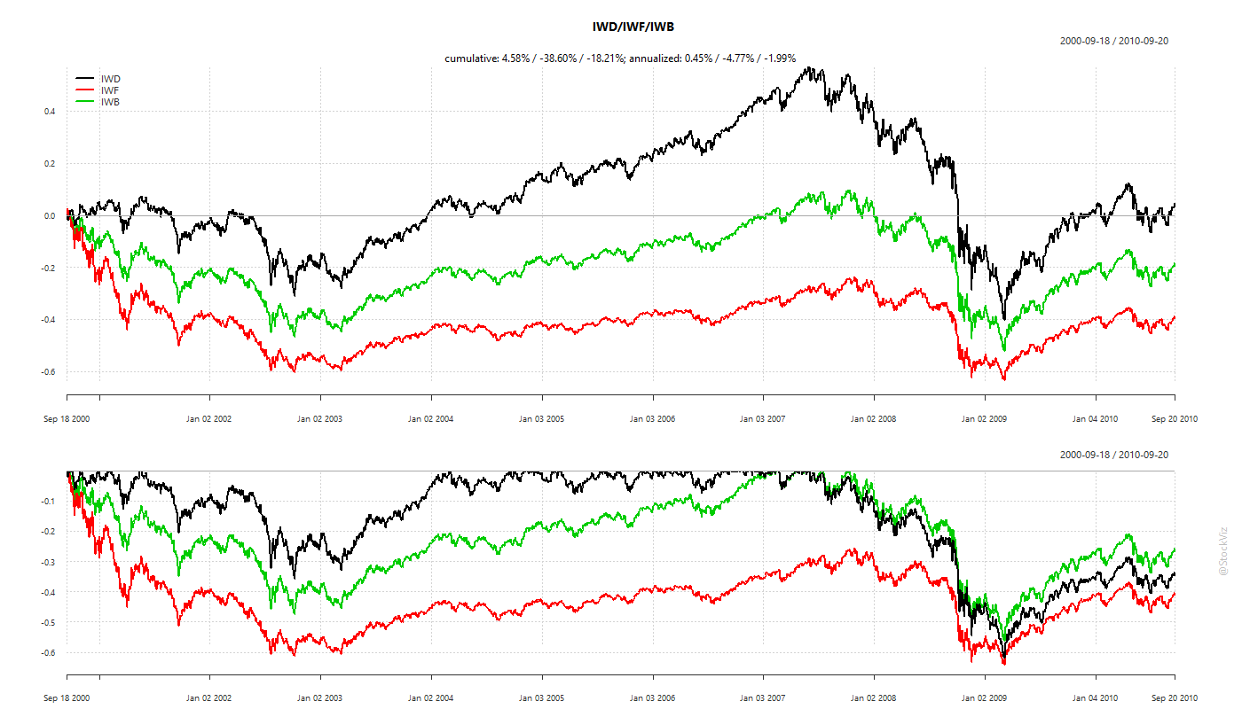
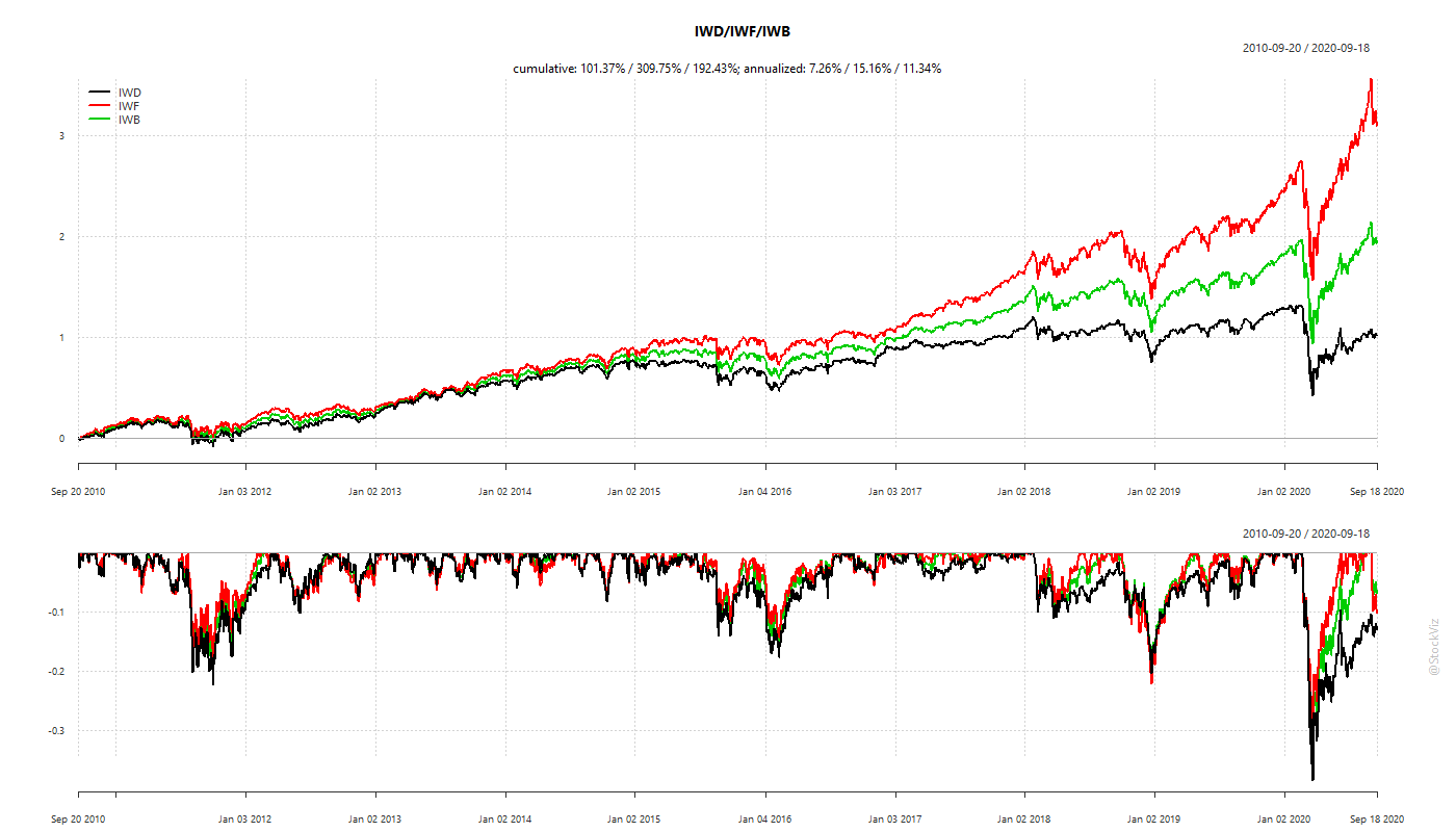
For example, Value vs. Growth.
Is Value/Growth Dead?
Consider IWD, the iShares Russell 1000 Value ETF, IWF, the iShares Russell 1000 Growth ETF and IWB, iShares Russell 1000 ETF.
2000 through 2010, value out-performed.
2010 through 2020, growth out-performed.
Whether you were a “Value” investor or a “Growth” investor, you saw 10-years (!) of under-performance.
Persistence of Out-performance
To avoid under-performing, an investor can:
Market-cap index (avoid choosing.)
Predict (good luck with that.)
Follow the herd (FOMO.)
Turns out, option #3 works pretty well and is robust.
Individual factors can be reliably timed based on their own recent performance.
Factor Momentum Everywhere – Tarun Gupta, Bryan T. Kelly (AQR)
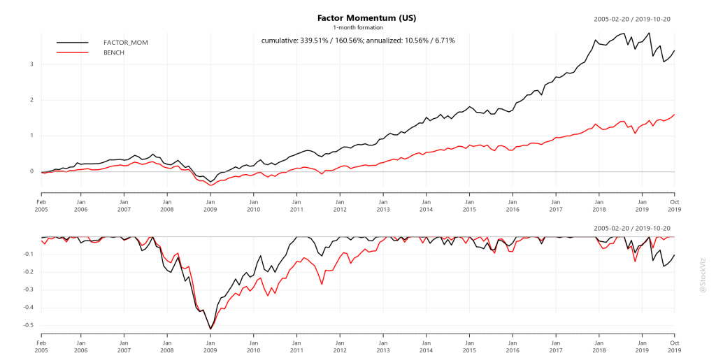
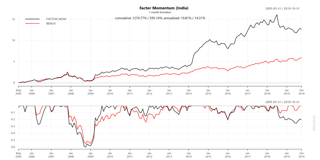
Rule: Buy whatever worked in the last month
Worked in the US
Worked in India
The problem, however, is that India has STT (Securities Transaction Tax) that the US doesn’t. And with a high turn-over strategy, STT can completely sap whatever alpha was produced.
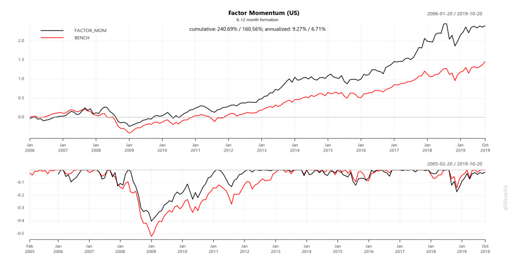
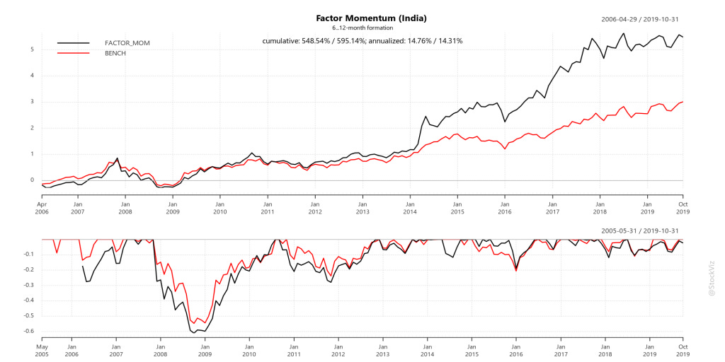
Rule: Buy the one with the Best Average Returns over the last 6-12 months
Worked in the US
Worked in India
Forward-Test
The back-test showed that for the US markets, investors can rotate into the factor that performed the best in the last month. And for India, investors can average into the one that had the best average 6-12 month returns.
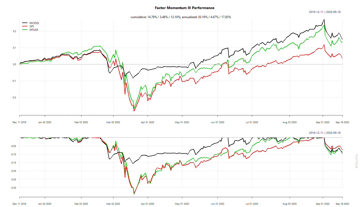
US
The Factor Momentum strategy beat plain-vanilla momentum (MTUM) and S&P 500 (SPY). It also avoided the Corona Cliff in March 2020.
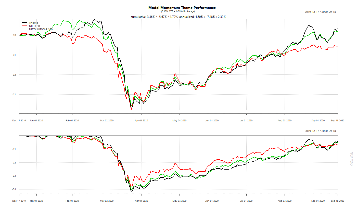
India
The Indian version of the Factor Momentum strategy is a mixed bag. Since it averages over a longer time-period, it is (understandably) slow to respond to sudden events. The dive during the Corona Cliff and subsequent performance is inline with the back-test. Thus far, it has marginally out-performed NIFTY 50 and MIDCAP 100 after STT and brokerage and we remain optimistic about its future.
Conclusion
Factor Rotation holds promise. Research, back-tests and forward-tests confirm. The trade-off is pretty clear as well: shorter look-backs/shallower draw-downs vs. transaction costs. Since trading US equities is nearly friction free, investors can use shorter look-backs. Indian investors will have to stomach deeper draw-downs given transaction taxes.
Our previous post on Momentum highlighted the inherent cliff-risk in the “buy-high, sell-higher” strategy. But even before Fama French published their 3-Factor paper, researchers had found that the “high risk = high reward” relationship is quite fragile. In 1972, Haugen, Robert A., and A. James Heins, studying the period from 1926 to 1971, came out with a working paper – On the Evidence Supporting the Existence of Risk Premiums in the Capital Market (ssrn) – that concluded that over the long run stock portfolios with lesser variance in monthly returns have experienced greater average returns than their ‘riskier’ counterparts (wikipedia).
Basically, a portfolio of low-volatility stocks will out-perform the market. More returns for less risk.
What Explains the Anomaly?
There are two main trains of thought on why this anomaly persists.
It is difficult to short high-beta stocks and buy low-beta stocks. Because, if it were easy, one could construct a zero-beta portfolio with positive expected returns… and this anomaly would vanish.
Stocks of companies with predictable earnings exhibit low-volatility. So, low-volatility is essentially high-quality – a known investment factor.
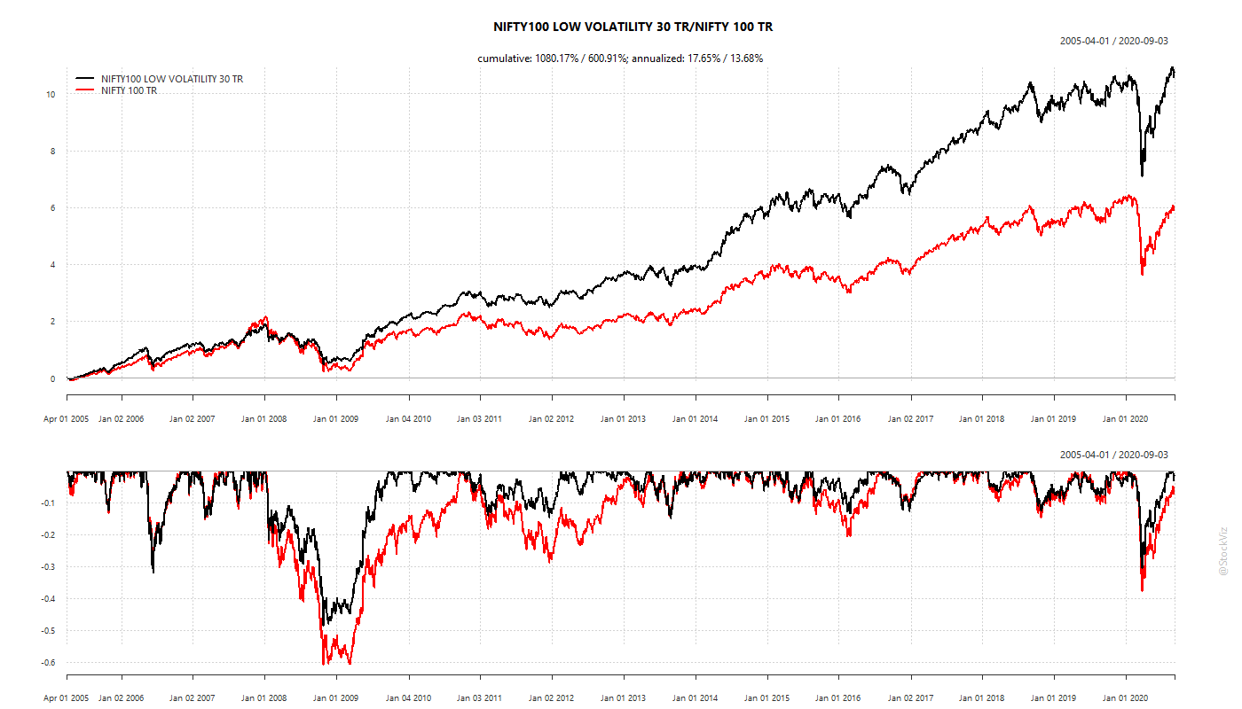
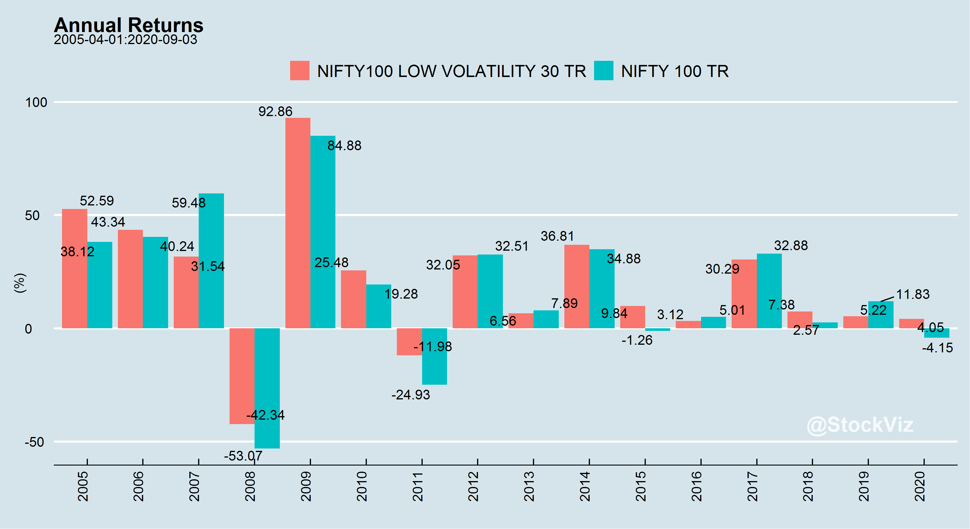
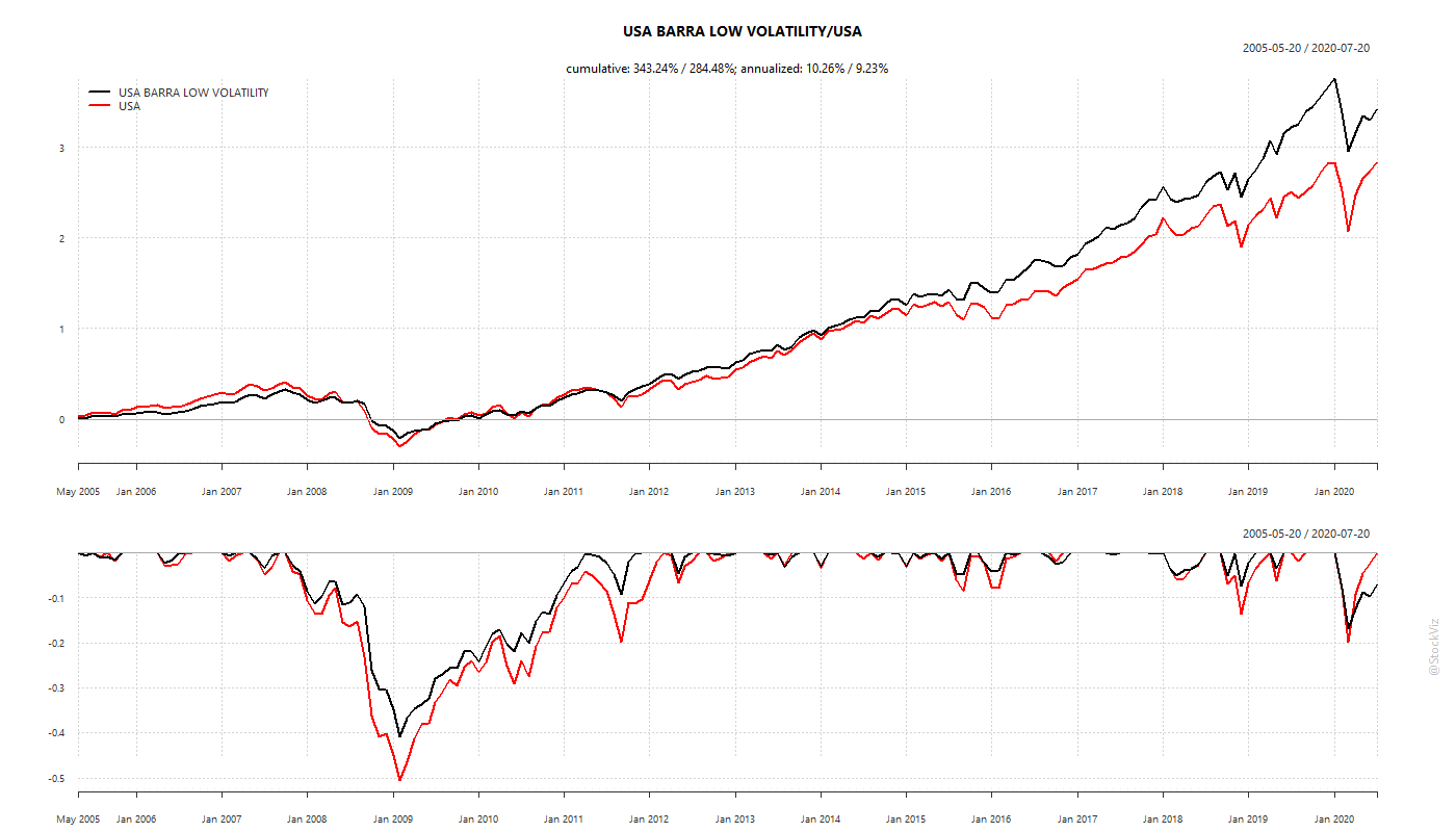
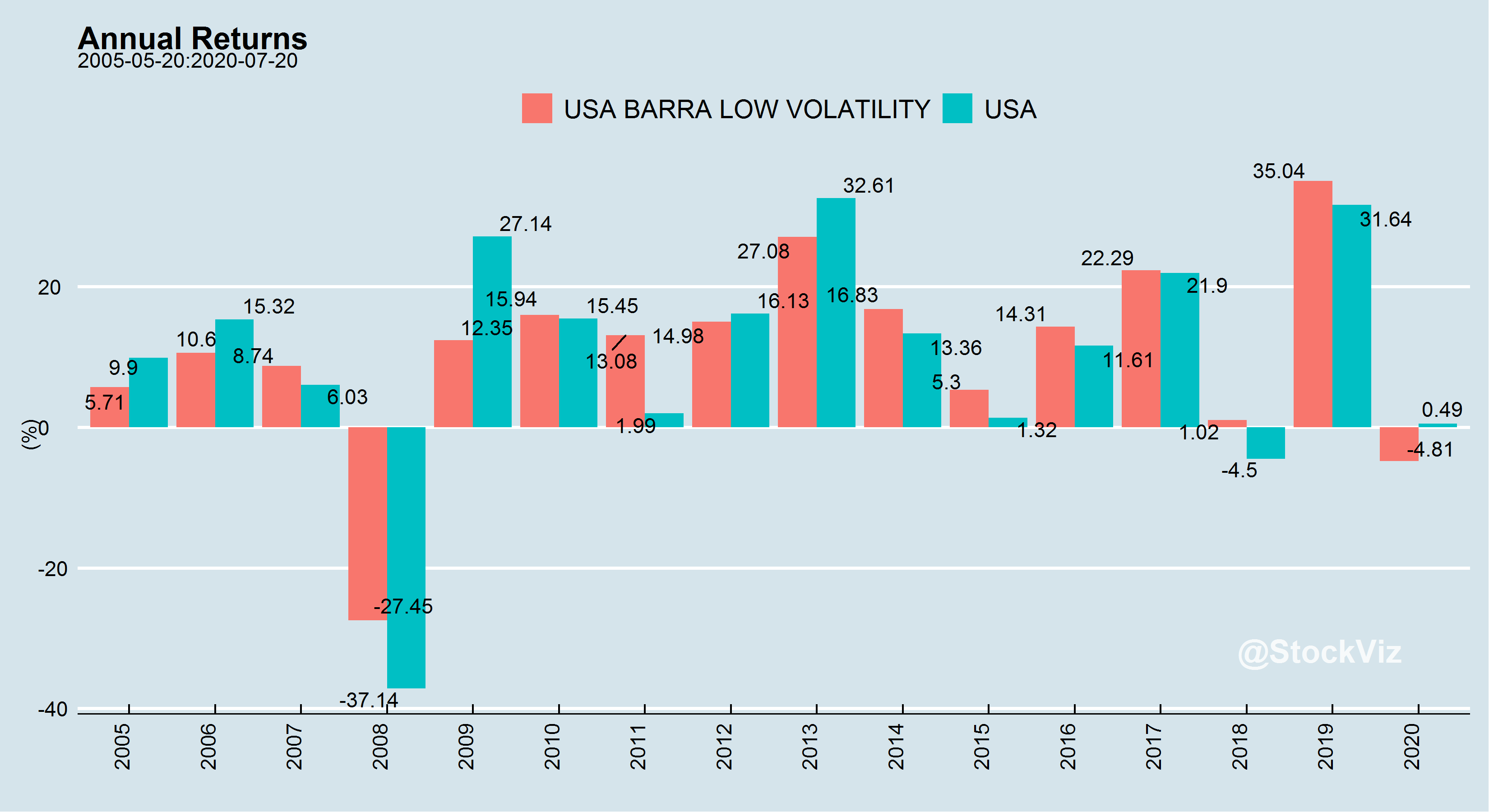
Historical Performance
While low-volatility has out-performed market indices, it is magic wand that makes drawdowns disappear.
India
US
Risks
The biggest risk in a portfolio of low-volatility stocks is that a large proportion of it could be held by weak hands – investors who are drawn to it primarily because of its low-volatility. And when faced with a drawdown that is steeper than historical experience, they can simultaneously head for the exits, resulting in a cascading drop in price. The triggers could be a missed earnings estimate, an industrial accident, etc. While momentum investors are used to being routinely hit in the head, a small shove can push low-volatility investors down a cliff.
Portfolio Construction
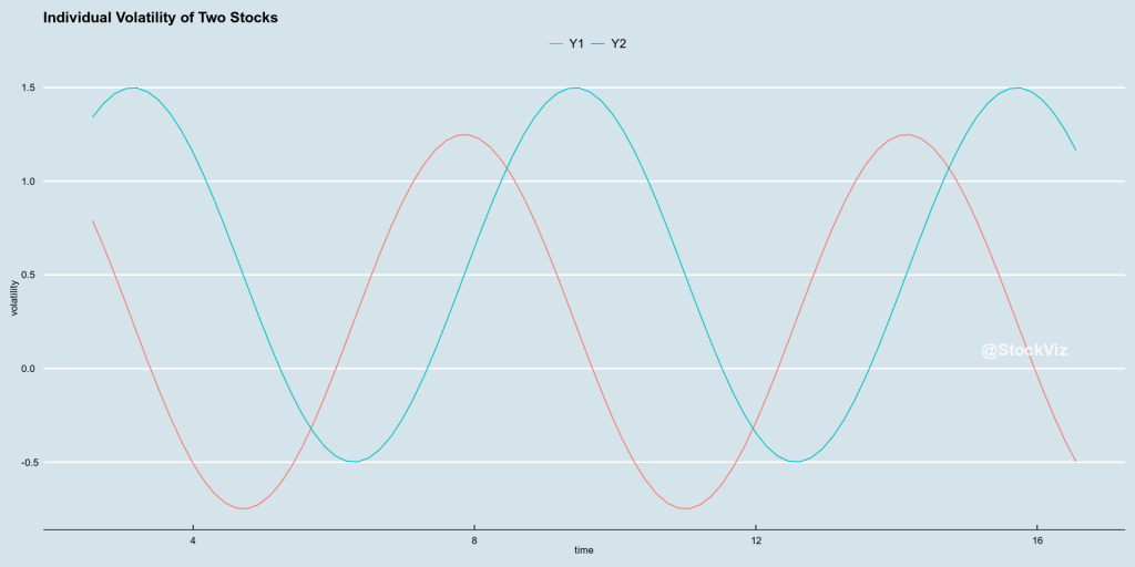
A portfolio of low-volatility stocks vs. a low-volatility portfolio of stocks.
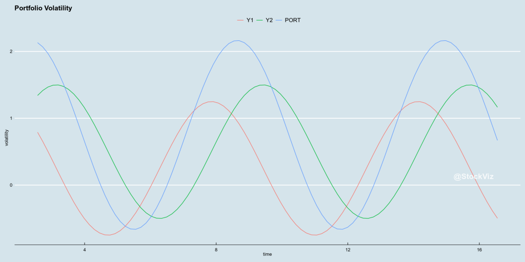
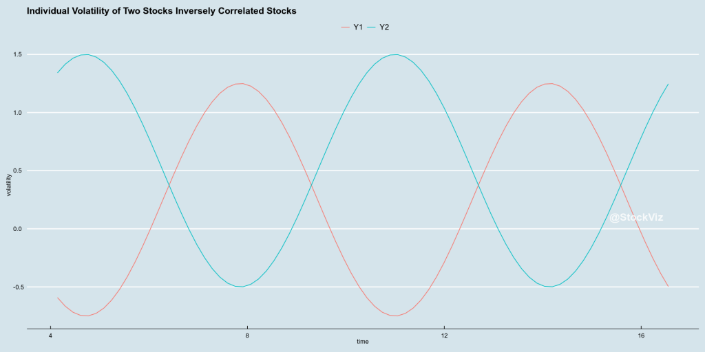
While initial research focused on stocks that had low-volatility, a collection of low-volatility stocks can result in a portfolio with high-volatility if the correlations among them are high. To illustrate, consider two low-volatility stocks who’s volatility varies through time like this:
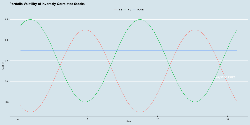
If you put them in the same portfolio, what happens to the portfolio volatility?
Now, what if you picked two stocks whose volatility were inversely correlate? In theory, you can mix to high-volatility stocks and get a low-volatility portfolio.
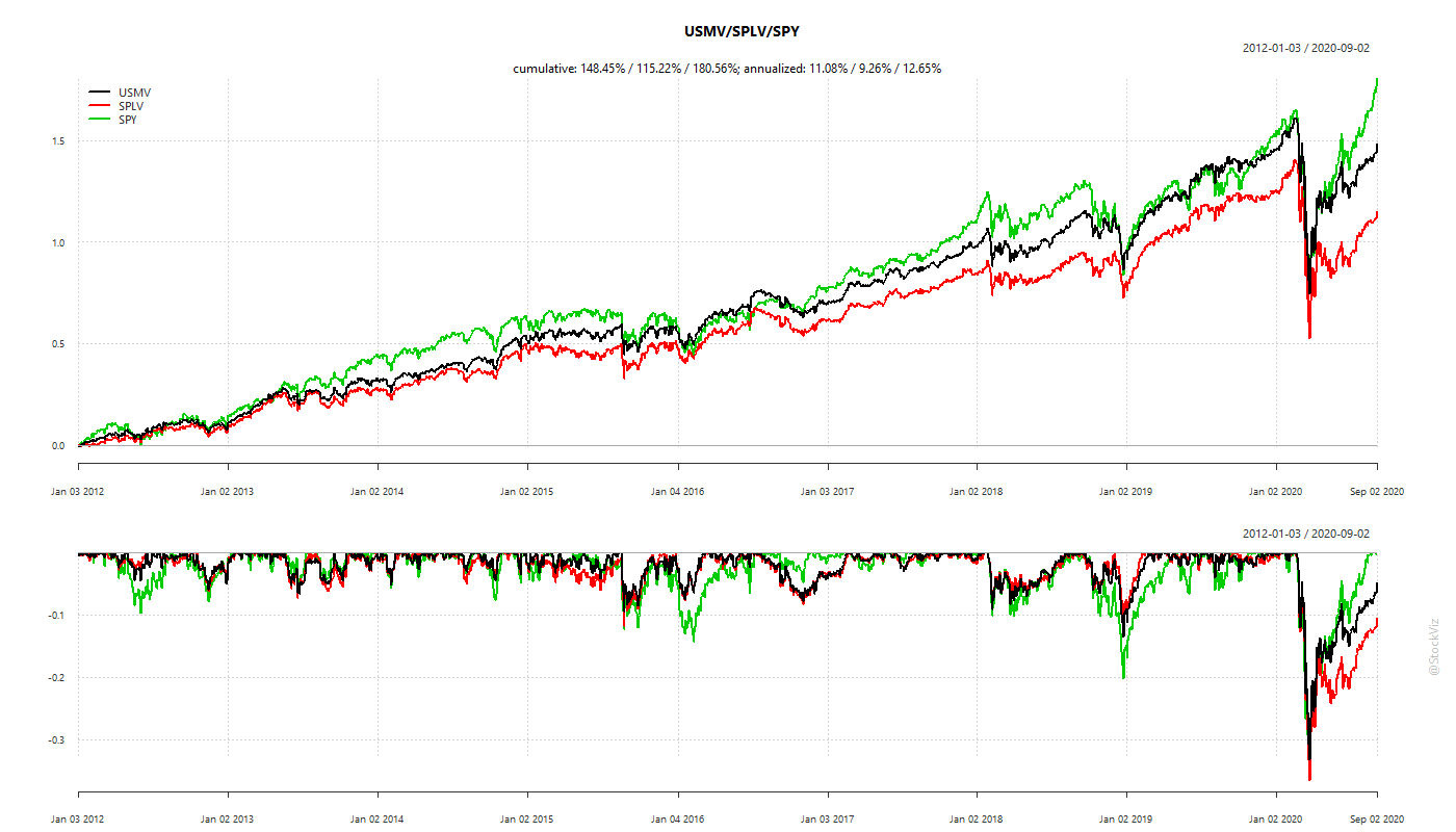
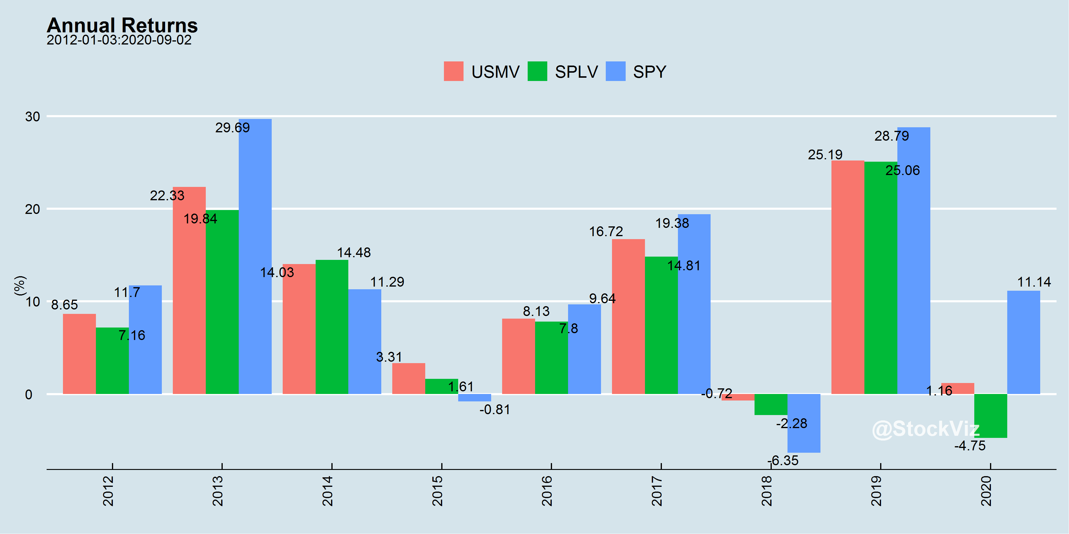
A Min-Vol portfolio tries to optimize the overall portfolio volatility. A completely different approach to having a portfolio of Low-Vol stocks. In the US, there are two large ETFs that track these different approaches: USMV – the iShares Edge MSCI Min Vol USA ETF, and SPLV – the Invesco S&P 500 Low Volatility ETF.
It appears that Min-Vol has an edge over Low-Vol in most scenarios.
Conclusion
While Momentum of Min/Low Volatility can appear to be diametrically different strategies, there are ways to mix them up in the same portfolio to achieve a lower-volatility momentum or a higher-return-low-vol outcomes.
However, at the end of the day, retail investors will forever be at the mercy of market beta. So, irrespective of which flavor of jam you like, the kind of bread you eat makes the biggest difference!
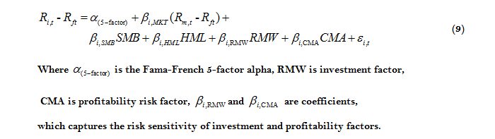
In our post on Intro to Factors, we showed how Fama and French added value (HML) and small-caps (SMB) to the original market-risk model to account for the relative out-performance of small-cap/value investment strategies. The genesis of their idea was basically that certain portfolio returns deviated significantly from the market-risk-only model and they wanted to see if they could account for it systematically.
In 2014, they updated their model by adding 2 more factors: profitability (RWM) and investment (CMA) – stocks with a high operating profitability perform better and stocks of companies with the high total asset growth have below average returns.
No Free Lunch
Investors can construct long-only portfolios with a single leg of any one of these factors to exploit it.
For example, one can rank stocks by high book-to-price ratio, take the first 100 of them and create a value portfolio. Such a portfolio will have a high factor loading (ß) for HML.
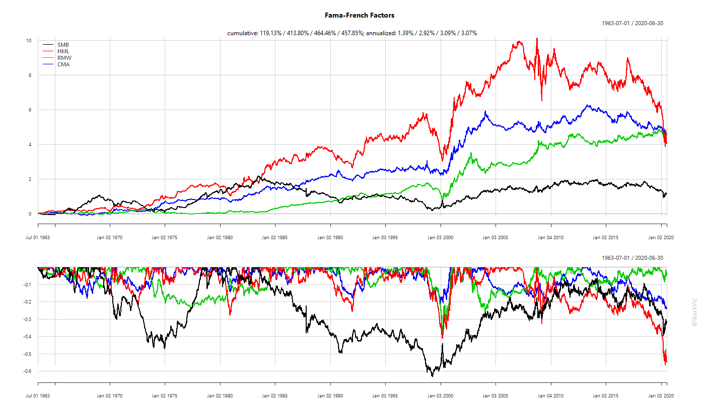
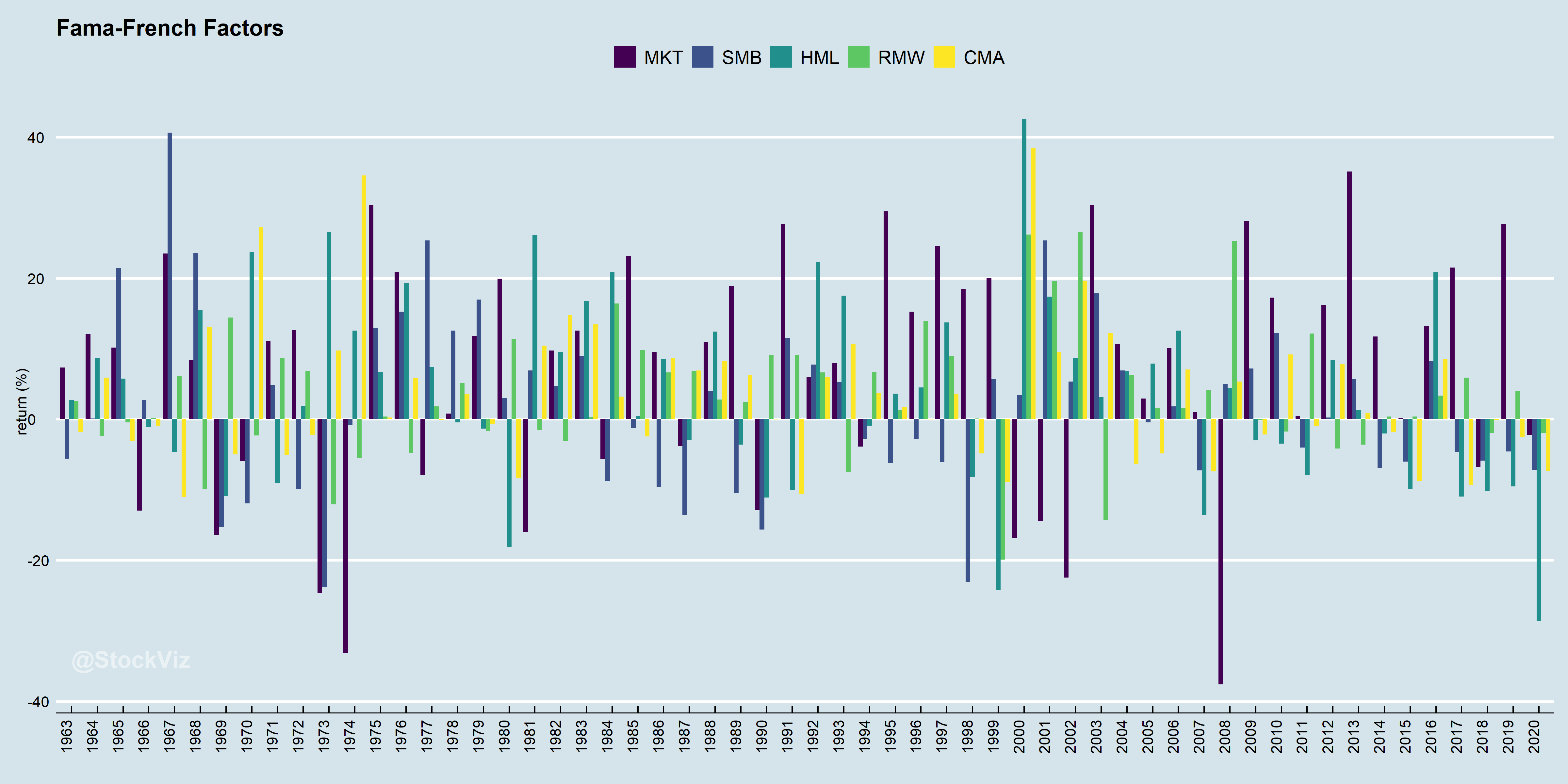
But just because you can do something like this, should you do it? Depends on your motivations. Factor returns ebb and flow. To visualize the cumulative effect of their spreads, you can plot them as a return series:
As you can see, single factors can spend years in negative territory. During that time, plain-old, low-cost market-beta would be racing ahead while a factor portfolio will be an expensive drag.
This leads us to posit that single factor portfolios are not buy-and-hold-forever investments. For example, during the final phases of a bull market, everything is expensive. So a portfolio of “pure value” stocks will be basically junk that no investor cares about. If you were to invest in such a portfolio, then when the market turns, these stocks are likely to drawdown way more than the rest of the market. If they were unloved in a bull, they will be massacred at the turn.
So unless you thoroughly understand the dynamics of how different factors behave in different market environments, you should stick to market beta.
The Factor Zoo
Fama and French opened the flood-gates for factor research. Academics rushed to discover and publish increasingly esoteric and often overlapping factors. At last count, there were over 400 factors published in various academic journals.
While some of them are a result of p-hacking and not all of them result in lasting alpha, there are a couple that have confounded academics and practitioners alike with their persistence: momentum and low-volatility.