Years of returns can get wiped out in a month in the markets. While investors mostly focus on the average, the tails end up dictating their actual returns. (Introduction)
Sampling and Measurement
Typically, a uniform sample is taken. The problem with this is it under-represents the tails. This leads to models that work on average but blow up on occasion. One way to overcome this problem is through stratified sampling. (Sampling)
Expected shortfall (ES) is a risk measure that can be used to estimate the loss during tail-events. (Measuring)
Acceptance
All assets have fat tails. It is a feature, not a bug. (Historical)
There is no asset free of extreme tail losses. If an asset produces any sort of return, it is going to be exposed to some sort of tail event.
One can try to find uncorrelated assets so that those losses don’t occur at the same time. However, correlations between asset returns are not stable – they change over time and behave quite erratically during market panics.
In the end, to be an investor is to accept the fact that large losses occasionally happen.
No matter how you slice it, there is no escaping tail events in investing. It is the nature of the beast and every attempt you make eliminating the risk results in you giving up a significant portion of your returns. But given two investment opportunities, how do you go about figuring out which one is more susceptible to tail events?
Expected shortfall (ES) is a risk measure that can be used to estimate the loss during tail-events. The “expected shortfall at q% level” is the expected return on the portfolio in the worst q% of cases. ES estimates the risk of an investment in a conservative way, focusing on the less profitable outcomes. For high values of q it ignores the most profitable but unlikely possibilities, while for small values of q it focuses on the worst losses. Typically q is 5% and in formulae, p (= 100% – q) is often used as a substitute.
ES of Weekly Returns
Here’s a dilemma that most investors face: Mid-caps have given higher returns in the past compared to large-caps. But, how do their tail-risks compare?
Turns out, ES of the NIFTY MIDCAP 150 TR index is -6.73% vs. NIFTY 50 TR’s -5.65%. This is how much an investor would have lost in the worst 5% of weeks since 2011.
Sampling
In our previous post, we showed how strata-sampling can be used to make sure that you don’t end up ignoring tail-risk in your simulations. By definition, tail-events are rare. So, the differences are subtle.
Tactical Allocation
Reducing tail-risk is one of the biggest draws of tactical allocation. Anything that reduces deep drawdowns has the effect of keeping investors faithful to their investment process.
One way to setup a tactical allocation strategy is to use a Simple Moving Average (SMA) to decide between equity and bond allocations. Different SMA look-back periods will result in different levels of risk and reward. From an ES point of view, here’s how things for NIFTY shakes out:
Since 1999
Since 2010
Using an SMA and re-balancing weekly significantly reduces tail-risk.
How far back should you go?
The problem with tail-events is that there aren’t enough of them to build an effective model. There’s always a temptation to use as much data as possible so that these events find sufficient representation. However, markets evolve, regulatory structures change and past data stop being representative.
For example, if you run a tactical allocation back-test with all the data that is available, you’ll conclude that shorter the SMA, the better:
However, if you remove 2008 and its aftermath and look only are the data from 2011 onward, you get a different picture:
While metrics like ES and strategies like SMA are useful, the data that they are presented will give different results based on the regime that they are drawn from.
Risk management is a continuous process and cannot be reduced to single number.
Often, the highest selling product is the one with the best narrative, not the one that provides the best value for money. Similarly, what drives eye-balls in media are narratives around “alpha,” “out-performance,” “best mutual funds,” “1% a day option strategies,” etc. But what really matters to you are things like “fund my kids’ college education,” “retire at a reasonable age,” “take a foreign vacation,” etc.
While it can be sexy to consider oneself as an investor – fantasizing belonging to the same tribe as Warren Buffett or Peter Lynch – people looking to meet goals that actually make a difference to their lives, are better off considering themselves as savers.
One saves their income to meet expenses in the future. Thinking this way drives focus towards the two things that are entirely within one’s control: savings rate and duration.
Once you shift the internal narrative to saving over investing, how you measure success changes as well. The last thing you’d want to do is play snakes-and-ladders with your portfolio. You’ll want to reduce risk as you get closer to withdrawal. And finally, you’ll realize that market’s return doesn’t matter as long as your funding needs are met.
Accepting lower returns
While you are stuck in Silk-Board traffic the next time, ponder this:
The current holder of the Outright World Land Speed Record is ThrustSSC driven by Andy Green, a twin turbofan jet-powered car which achieved 763.035 mph – 1227.985 km/h – over one mile in October 1997.
How come you don’t drive a jet-powered car? Wouldn’t that be the “best” car?
The reason why you drive a mini-van and not a jet is because your life involves mundane things like grocery shopping, dropping your kids off to school, going to the mall, etc.
Similarly, your portfolio should reflect your life. Just like you make-do with a mini-van (not the fastest, not the sexiest, but practical,) you should construct a portfolio that gets the job done. And that often involves not being the “best” investor but focusing on risk.
Managing risk means accepting that you will never go as fast as Andy Green.
Market returns vs. Portfolio returns
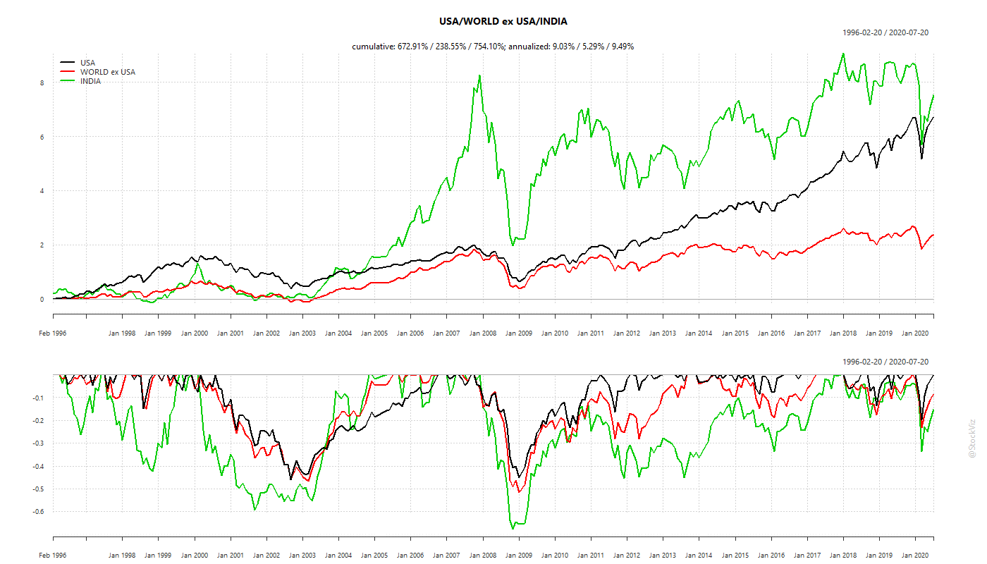
A “lost-decade” for stocks probably happens every decade.
Here’s MSCI indices for US, Developed Markets ex-US and India. The only thing that can be said for certain is that stocks fluctuate and occasionally tank 30-40% and sometimes even 70%
If you only invested in stocks and you needed money to send your kinds to college in 2008, then, well, good luck!
A goal-oriented portfolio constructed with this in mind will necessarily under-perform an all-stock portfolio when stocks are screaming higher. It will also not go down in flames when stocks tank, as they very often do. So, market returns ≠ portfolio returns.
Take risks when you can, not when you have to
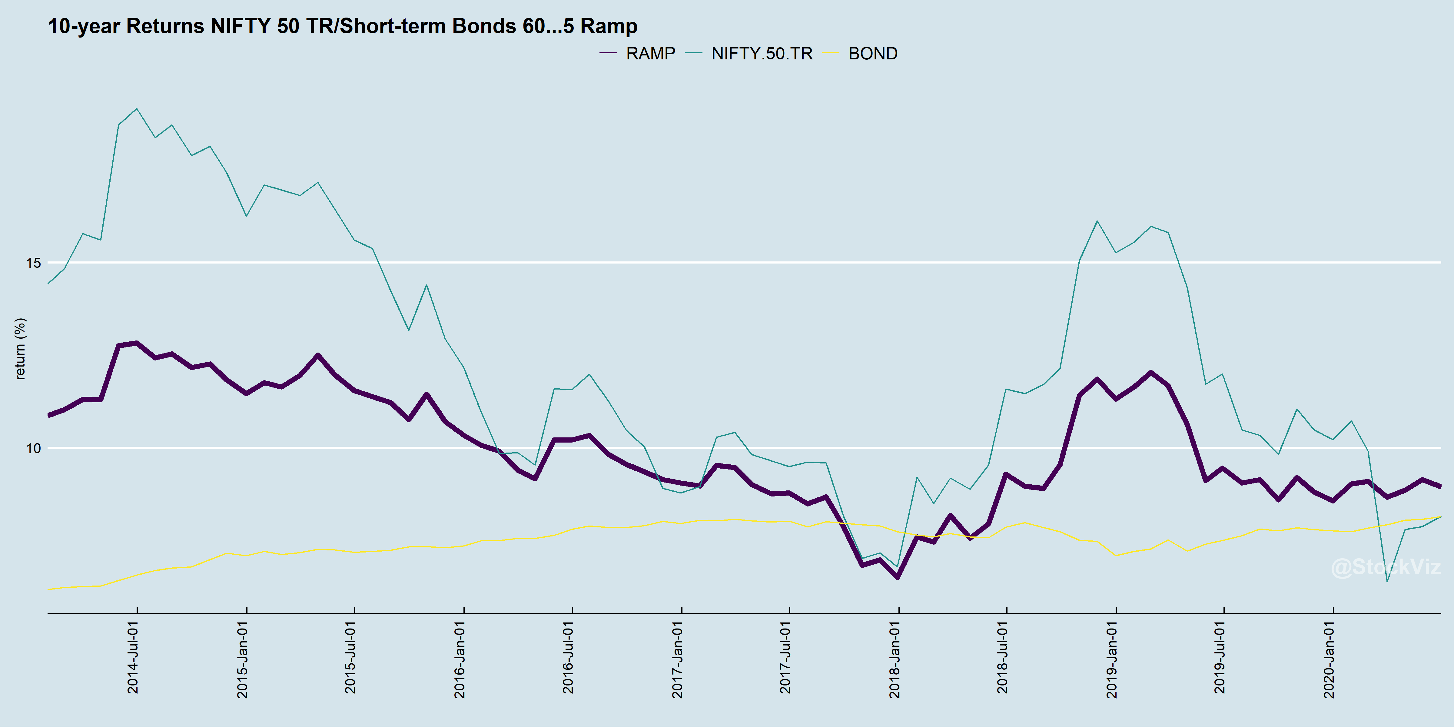
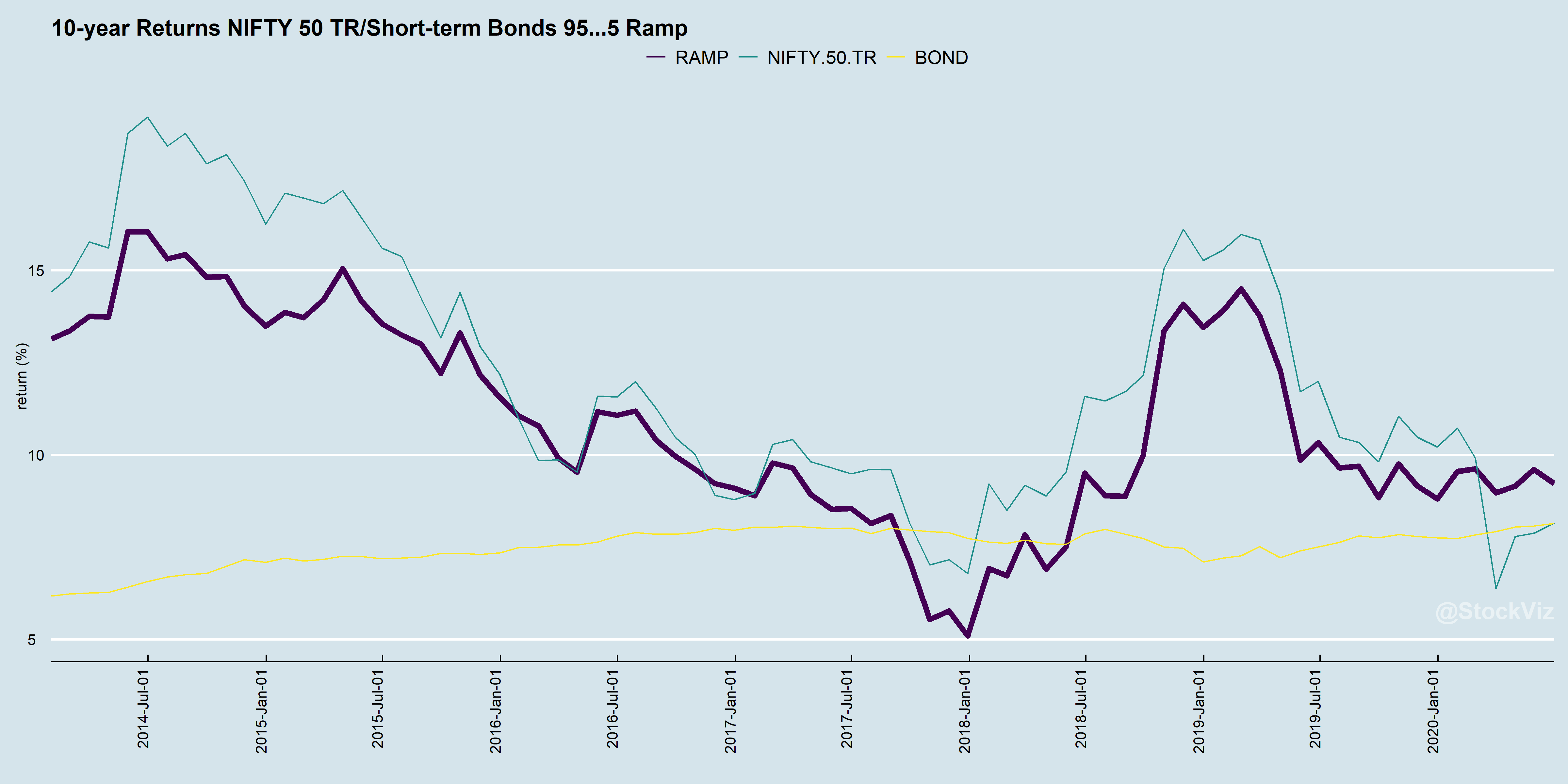
If you are saving for a goal 10 years away, it is safer to bet that markets will recover in 10 years than to bet that they will recover in one. So it maybe a good idea to load-up on risk at the beginning and slowly de-risk as time goes on. In fact, if you don’t take risk upfront, then you maybe doing it wrong.
Here’s the difference between starting at 60% NIFTY vs. 95% and slowly ramping down over 10 years:
Glide path and Target-dates
The strategy described above is an example of a 10-year target-date fund with a linear glide-path. You start with an allocation that you are comfortable with – can be anything from 60/40 through 95/5 split between equities and bonds – and then every month nudge it so that at the “target-date” the allocation becomes 5/95. It is a way of taking risks upfront and de-risking the portfolio as the withdrawal date gets closer.
For longer time-horizons, say 30 years, you can also look at an exponential glide-path. The basic concept remains the same: reduce risk as you get closer towards withdrawal.
While decidedly unsexy, this “mini-van” strategy will safely get you and your family where you need to go.
While developing a model, historical data alone may not be sufficient to test its robustness. One way to generate test data is to re-sample historical data. This “re-arrangement” of past time-series can then be fed to the model to see how it behaves.
The problem with sampling historical market data is that it may not sufficiently account for fat-tails. Typically, a uniform sample is taken. The problem with this is it under-represents the tails. This leads to models that work on average but blow up on occasion. Something you’d like to avoid.
One way to overcome this problem is through stratified sampling. You chop the data into intervals and use their frequencies to probability weight the sample. This preserves the original distribution in the sample.
Notice the skew and the tails in the “STRAT” densities for both NIFTY and MIDCAP indices. This distribution is far more likely to result in a robust model compared to the one that just uses uniform sampling.