Tag: allocation

Volatility and Allocation

Think in terms of volatility buckets, not assets

This post is part of our series on diversification and asset allocation. Previously:

  1. Diversification and its Malcontents

  2. The Permanent Portfolio

  3. Sequence Risk and Asset Allocation

  4. Static vs. Tactical Allocation

  5. Tactical Allocation


The thrust of our previous posts on allocation was that Indian investors shouldn’t blindly copy strategies that worked well in the US. There are a lot of qualitative arguments to be made to support a India-dominant view for allocation strategies. In this post, we introduce a quantitative aspect to the discussion.

It is Volatility, Stupid!

In finance, more than any other field, it is very easy to get correlation and causation mixed up.

A man goes to the doctor and says, “Doctor, wherever I touch, it hurts.”
The doctor asks, “What do you mean?”
The man says, “When I touch my shoulder, it really hurts. When I touch my knee – OUCH! When I touch my forehead, it really, really hurts.”
The doctor says, “I know what’s wrong with you. You’ve broken your finger!”

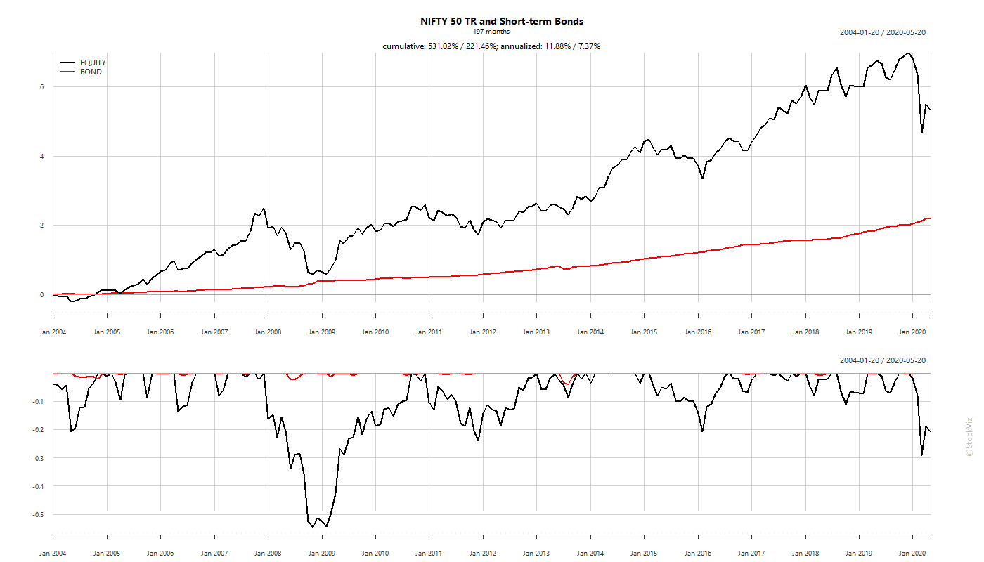
There are no universal laws for an asset class that holds across geographies and economic systems. The reason why a 60/40 Portfolio “works” in the US has more to with the quantitative aspects of the assets being mixed than what they are called. US bonds have benefitted greatly from a 30 year slide in yields, benign inflation and a flight-to-safety bid. None of these hold true for Indian bonds. So, expecting a 60/40 Indian portfolio to behave like a 60/40 US portfolio just because you mixed the same assets together is idiotic.

The most import aspect while considering assets for diversification are their volatilities. Specifically, the correlation of their volatilities at their left tails.

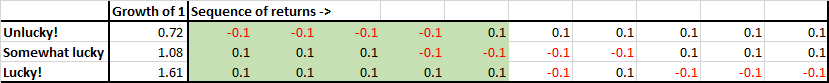
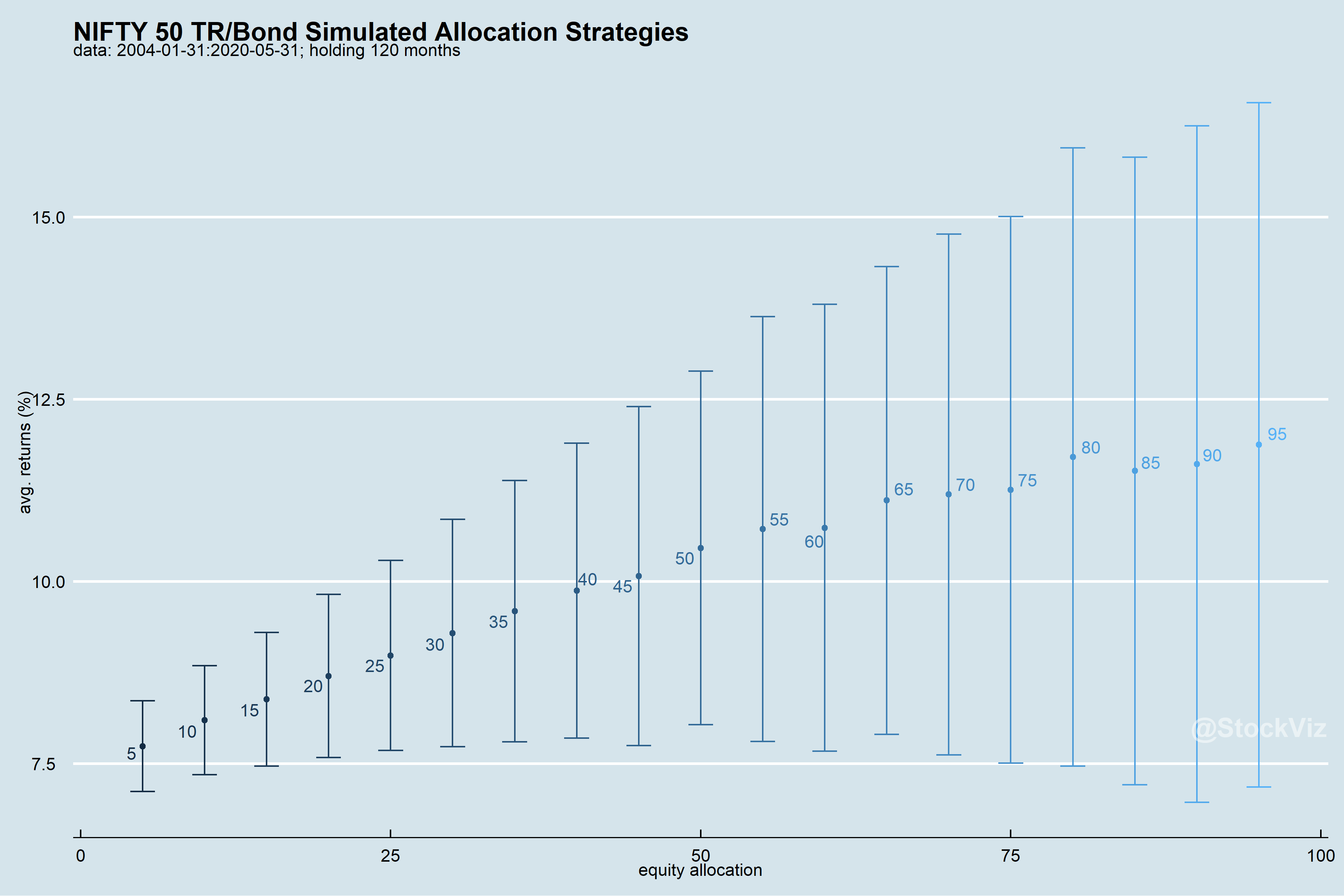
To keep things simple, consider a 2 asset portfolio: Eq and X. Eq has some average return that will be held constant during this analysis. What changes is its standard deviation (aka, volatility.) X is a stable asset with zero volatility (think of it as a fixed deposit.) How does different allocations to Eq change portfolio returns and volatility?

  1. Low volatility is supportive of higher allocations

  2. Higher allocations to the higher volatility asset progressively reduces the predictability of portfolio returns

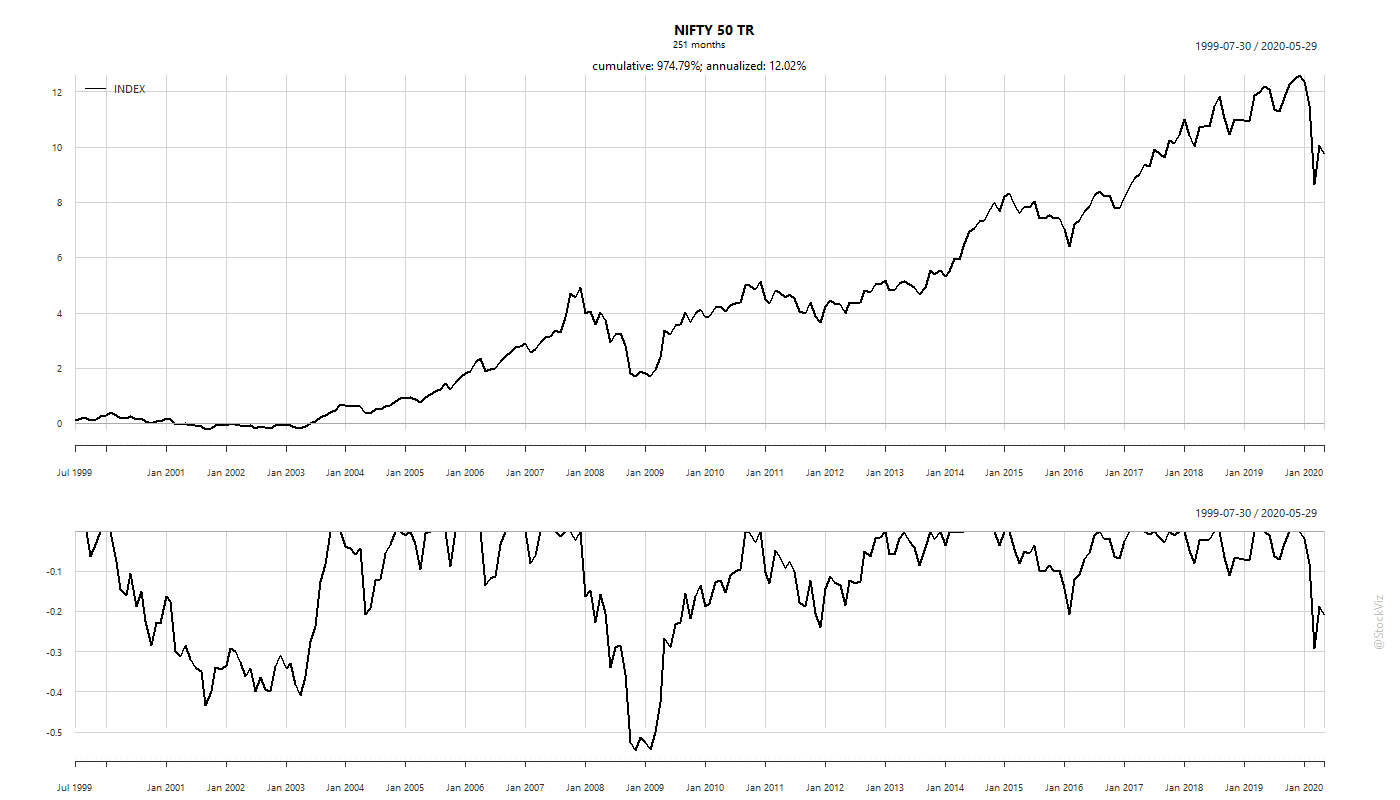
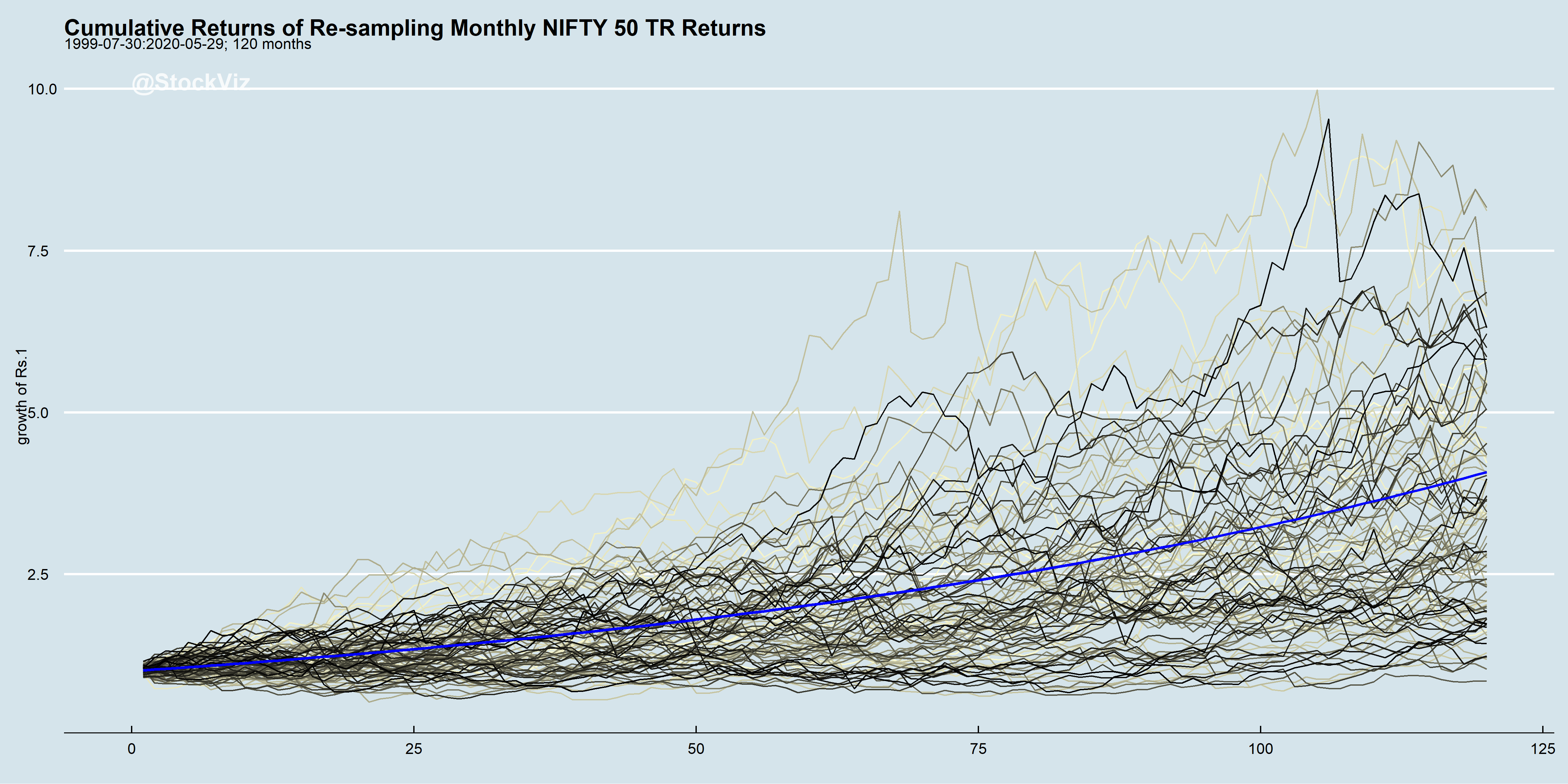
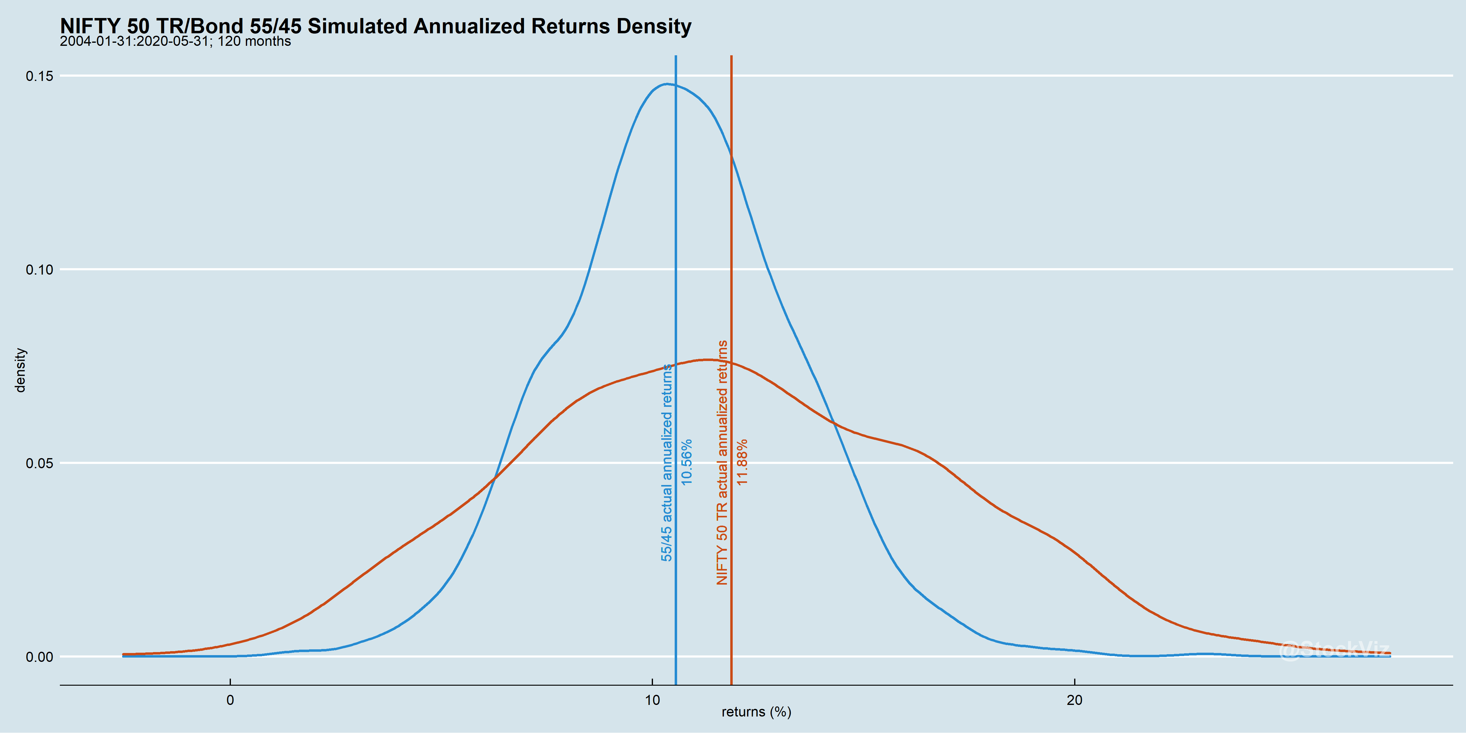
Volatility is Volatile

Asset return volatility is itself volatile.

The past performance of a diversified portfolio is based on the realized volatility of its components. However, volatility itself is unpredictable over long periods of time.

Take-away

While considering assets to diversify into, look at the volatility of the asset rather than what it is called.

Don’t expect the quantitative aspect of an asset class to transcend economic systems – different markets need different treatments.

All investing is forecasting. And all allocation is forecasting volatilities.

The Permanent Portfolio

Pain is eternal

This post is part of our series on diversification and asset allocation. Previously:

  1. Diversification and its Malcontents

  2. Sequence Risk and Asset Allocation

  3. Static vs. Tactical Allocation

  4. Tactical Allocation


The Permanent Portfolio – an equal weighted allocation to stocks, bonds, gold, and cash – was devised by free-market investment analyst, Harry Browne, in the 1980s. The basic idea is that no matter what the macro environment, the portfolio will not totally crash and burn.

The American Experience

Turns out, the theory largely worked for US investors.

If you look at the rolling 3-year annualized returns of the Permanent Portfolio, never has it given negative returns. In sharp contrast to equities and gold, US bonds have been spectacularly stable. So naturally, an equal weighted allocation to all for assets delivered decent returns with low drawdowns.

Did it work for Indian Investors?

Indian investors need to be careful with their bond allocations.

The Permanent Portfolio allocates 50% towards fixed income. This is a problem for Indian investors because unlike US bonds, Indian bonds do not have a “flight to safety” bid – they tank along with stocks during market panics.

A density plot of annualized 3-year rolling returns highlights the left-tail problem with the Indian Permanent Portfolio:

Take-away

Beware of people preaching simple solutions to complex problems. If the answer was easy someone more intelligent would have thought of it a long time ago – complex problems invariably require complex and difficult solutions. – Steve Herbert

This is another instance of a “copy-paste” solution disappointing Indian investors.

The common thread connecting the misfiring of the 60/40 and the Permanent portfolios is the vastly different paths taken by Indian bonds. Is there a better way to crack this nut? Stay tuned.

Decoding the 60/40 Portfolio

Get onboard with the embedded assumptions before diving head-first.

The 60/40 allocation – 60% in equities, 40% in bonds – is the bedrock on which most portfolios in the US are built. Jack Bogle was its biggest proponent and it serves as a benchmark in most portfolio discussions.


This post is part of our series on diversification and asset allocation. Previously:

  1. Diversification and its Malcontents

  2. Sequence Risk and Asset Allocation

  3. Static vs. Tactical Allocation

  4. Tactical Allocation


Historical Performance

From a cumulative performance point of view, it is easy to see why it is attractive.

Even with an annual rebalance, the 60/40 delivered. How did it achieve this remarkable feat? Should investors expect similar magic with the same allocation to Indian equities/bonds?

The biggest difference: Volatility

Ever since Volcker got done slaying inflation in the 80’s, US bond yields have been on a secular decline with declining volatility and increasingly occupying the place of a “flight-to-safety” asset.

Indian bonds, however, are in no way comparable to US bonds when it comes to volatility.

Volatility of US Bond returns (3-year, rolling) with those of Indian Gilts:

On a cumulative basis, Indian bond investors have taken a lot of pain for a 50bps out-performance.

Indian bonds haven’t exactly acted as a safe-haven in times of stress for Indian investors. Adding equities into the mix brings out the extreme volatility of Indian stocks:

However, the silver-lining is that Indian asset volatility have been moderating since 2015.

The 60/40

Over a long enough timeline, it looks like the 60/40 should work in India as well.

But, what if, most of the long-term returns that can be seen since 2000 was front-loaded? Rolling-returns over different windows should give us an idea:

The 5-year window shows returns stabilizing around an average of 5% (in USD.)

Embedded forecasts

All investing is forecasting. As much as one would want to follow a 60/40 allocation for its popularity, it behooves to ask: what are the embedded forecasts about Indian equities and bonds in such a strategy?

  1. Bond volatility will continue to go down.

    • The market will continue to deepen.

    • Inflation will be range-bound.

  2. Equities will be loosely efficient.

    • The gap between growth assumptions and equity valuations will be within a gradually tightening band.

  3. Ease of doing business:

    • Contract enforcement

    • Flexible labor laws

    • Infrastructure

    • Bankruptcy protection and resolution

    • Policy stability

Basically, India will move towards an environment with a predictable tax regime, a rules-based fiscal policy, and regulations that are fair and strictly enforced.

Take-away

There are millions of permutations and combinations of securities for investors to allocate. The question that every investor should ask themselves is how much time, effort and money they are willing to spend chasing returns that beats low-cost, set-it-and-forget-it strategies like the 60/40.

If you are in investor who craves simplicity & low-cost and your beliefs about the future is mostly in line with the assumptions presented above, then this is the strategy for you.

Static vs. Tactical Allocation

What makes sense and for whom.

Our first post discussed one of the biggest risk that investors face: sequence-of-returns risk. One way to mitigate this is through asset allocation. You can just put half your investments in equities and half in bonds to reduce your over-all risk. An alternative is tactical allocation. In tactical allocation, you use a signal, like an SMA (Simple Moving Average) or equity valuations to switch between equities and bonds. Here, at any given point in time, you are fully invested in one asset class.

So, which one is “better?”

The answer is, “it depends!”

It depends on the investor’s tax slab and whether it is going to be a lump-sum investment or a SIP. For lump-sums, investors are better off with a tactical approach (bonus if you are in a lower tax slab.) For SIP investors, static allocation makes more sense because you can maintain proportions without selling the over-allocated asset. And, surprisingly, the frequency of re-balance did not matter for static allocation.

Re-balance Frequency for Static Allocation

Our back-test shows that there is no difference to overall returns between monthly and annual re-balance frequencies. Focus on the black line on the following charts.

Monthly re-balance:

Annual re-balance:

Static vs. Tactical – Rolling 10-year Returns

Static allocation returns have been converging with those of the tactical strategy.

Green: static 50/50 allocation, monthly re-balance

Red dot: static 50/50 allocation, annual re-balance

Brown: 50-day SMA, weekly sampling

The above chart reinforces a couple of points we made earlier:

  1. Sequence-of-returns risk is real.

  2. Large impact of when you start and stop your investments (“luck” factor,) is real.

  3. Excess returns in a back-test could be because of high transaction costs or lack of liquidity. In such cases, expect excess returns to diminish as those factors improve.

  4. Barring a couple of instances, annually re-balanced returns were within the range of those that were re-balanced monthly.

Tax impact

If you do a worst-case tax impact analysis on both static vs tactical (SMA) strategies, over the long-arch of time, tactical wins. In the chart below, static allocation is the ALLOC.NET-ST (green) line and tactical is the SMA.NET-ST (red) line.

However, if you are a SIP investor, then you don’t need to sell the over-allocated asset under a static-allocation setup – you could just buy the under-allocated one till it falls back in line. So, if you plot the after-tax returns of tactical allocation with pre-tax returns of static allocation by year:

Years 2011 through now, there is hardly any difference between them. They both turn in annualized gains in the low 7% range – adding about 1.25% over an all equity portfolio.

Summary

  1. For lump-sums, choose tactical. For SIP choose static allocation.

  2. Don’t ignore bonds. There are periods where a bulk of the returns are driven them.

  3. Don’t ignore the role of taxes in DIY. For example, a mutual fund that wraps the SMA strategy would enjoy a 2+ % boost in annualized returns.

Mitigating Sequence Risk through Asset Allocation

Sequence Risk (sometimes called sequence-of-returns risk) is the effect that the order of returns has on a portfolio.

For example, say you look at NIFTY and find that it gave negative 10% returns 4 years out of 10, and the rest of the years it gave positive 10% returns. You want to be invested for 5 years, so you expect 2 of those years to be negative. Sequence risk means that it is possible that you could have all of those negative 4 years during the 5 year period that you have invested.

The order in which losses occur impacts the portfolio’s terminal value

The annualized return of the NIFTY 50 TR index, since inception through May-2020, is roughly 12%. However, it has not been without periods where it was down over 50%.

NIFY 50 TR cumulative returns since inception

The lower part of the chart shows the drawdowns that have occurred in the past. Sometimes, it has taken years to recover from losses. The problem is that most investors have a pre-defined time-frame in mind. They want to be invested, say, for 10 years. Not “forever.” This is where sequence risk becomes a problem.

For a 10-year period, if you re-sample the monthly returns of the NIFTY 50 TR index and re-construct a return time-series, say, a 100 times, and plot the cumulative returns of each, it looks something like this:

The blue line is the “average” monthly return compounded for 10-years

Put another way, there is a non-trivial chance that an investor could end up with negative returns in a given 10-year period even if NIFTY’s return distribution did not change.

So, what is an investor to do? There are two approaches that have known to work:

  1. Diversification. Allocate to non-correlated assets.
  2. Get Tactical. Markets are known to trend. Try and preemptively exit from assets who’s prices are trending down.

There are a million different ways to skin each of these approaches. The simplest one is to add bonds to the portfolio.

NIFTY 50 TR and 0-5yr TRI

Bonds, especially sovereign bonds (issued by stable countries, of course) have very low drawdowns. So when you combine it with equities, you end up with a lot less sequence risk than pure equities.

If you simulate different proportions of equities and bonds and plot them along with their standard deviations, you’ll get an idea of where to trade-off stability with returns.

Trade-off between risk and returns

Let’s say that the sweet-spot is equity/bond ratios with avg. returns more than 10% but lower-bounded at 7.5%, you get 45/55, 50/50 and 55/45 as ideal allocations. While a 60/40 equity/bond allocation is the go-to for most advisors, there is no reason why it can’t be a more conservative 45/55.

Cumulative returns of different allocation ratios

Note the lower drawdowns of diversified portfolios. While the equity-only portfolio would have had an annualized return of 11.88% during the period, diversified portfolios ranged from 10.10% – 10.56%. The trade-off is that diversified portfolios have vastly less sequence risk.

The left-tail has been flattened while returns are now clustered more towards the average

Diversification changes the shape of the return distribution so that an average investor has a greater probability of experiencing average returns.

Read more about portfolio allocation across different assets here.

Code and images are on github.