We are setup for an epic fight between Amazon and Alibaba in the US. Something that will be keenly watched by the Bansals, now that they want to be Alibaba instead of Amazon (LiveMint). But what exactly is Alibaba? How did they become a multi-billion dollar company with a finger in every pie?
Alibaba is a lot of different things for different people
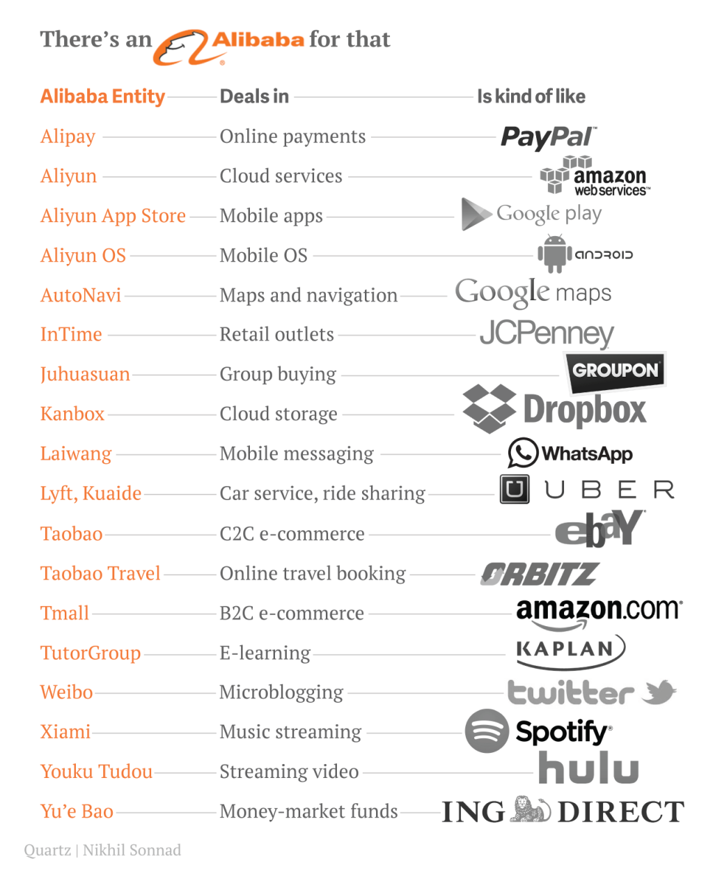
If you think it looks like a land-grab, you are right. They basically asked: What would a newly online Chinese consumer want? And connected the dots.
Alibaba is huge
The Wall Street Journal says that Alibaba’s Taobao and Tmall sites reached $240 billion in combined transaction volume last year. By way of contrast, EBay posted $76.5 billion last year in so-called “gross merchandise volume” excluding vehicles.
Alibaba now handles roughly 80% of all online shopping in China. Alipay is not only a payments processor (the world’s largest, at that) but also runs a money-market fund with more than $65 billion in assets.
What are investors buying?
Its hard to say. Alibaba stock will buy investors a stake in a Cayman Islands-registered entity which is under contract to receive the profit from Alibaba’s lucrative Chinese assets but will not actually own them.
The reason is that China permits privately controlled firms in some industries to tap foreign markets by establishing offshore companies permitted to wholly own Chinese companies. Yet it prohibits foreign investments in certain restricted industries, including the Internet. These controlled industries must be owned by Chinese nationals; no foreign investment are allowed.
So, the work-around has been to establish ownership by Chinese nationals, while setting up an offshore company that can be publicly listed. Mimic an owner relationship by setting up contracts between the two parties so that the offshore public firm reaps the successes of the Chinese firm — without actually owning shares in it.
Basically, investors are buying into a story.
Can Flipkart + Myntra = Alibaba?
Hard to say. Social networking in India is basically owned by Facebook (+ WhatsApp). Uber is here, and so are half a dozen home-grown taxi “startups.” Online payments are heavily regulated by the RBI and payments startups are in round 2 of the hunger games. Amazon.in is a looming threat and selling other people’s brands is a lousy business model. Its probably too late to be the “Alibaba of India”… and its probably going to be tougher just hanging on to being the “Amazon of India.”
Besides, isn’t “______ of [something]” a red flag for most venture capital firms? But it seems like its a story that investors are willing to hang their hat on for now.
Sources: