Category: Investing Insight

Investing insight to make you a better investor.

Long term ≠ Always

always2

Previously, we had highlighted the difference between ‘Long-Term Investing vs. Buy And Hold Forever’ (src) Economies shift, competition catches up, moats wither away. So it is essential to have a periodic review of your portfolio.

Recently, in a post titled ‘The answer is that there is no answer’ (src) we saw the inherent contradictions that exist in asset management.

James Osborne over at Bason Asset Management brings it together brilliantly:

The world is a complex place and how each generation of investors experiences these long term truths may be very different. This is simply a reminder that in some periods, we may have a different experience than these long-term facts.
 
Most importantly we should be aware that “over the long term” doesn’t mean “always” in advance so that we aren’t surprised when we experience the opposite result of our long-term beliefs.

The whole thing is worth a read.

Source: “OVER THE LONG TERM” DOESN’T MEAN “ALWAYS”

Understanding Nifty Volatility

Definition

Volatility (σ) is a measure for variation of price of a financial instrument over time. Historic volatility is derived from time series of past market prices. There are different ways of calculating volatility. At StockViz, we use Yang Zhang Volatility.

σ is one of the biggest contributor of option premiums. Understanding its true nature will help you trade it better.

Volatility spikes

Observe the volatility spikes since 2005. Even though the average is around 0.3, its not uncommon to have huge swings.

nifty-volatility

Fat tails abound

nifty-volatility-10-histogram

nifty-volatility-20-histogram

nifty-volatility-30-histogram

nifty-volatility-50-histogram

Trading strategy

Always try to be on the long-side of volatility. It might be tempting, while trading options, to try and clip the carry on θ-decay. But you should always be aware of the fat-tails of volatility that can crush many months of carry P&L overnight.

The most important assumption

Prices and Returns

Prices don’t follow a statistical distribution (they are not ‘stationary’.) There is no obvious mean price and it doesn’t make sense to talk about the standard deviation of the price. Working with such non-stationary timeseries is a hassle.

NIFTY 2005-2014

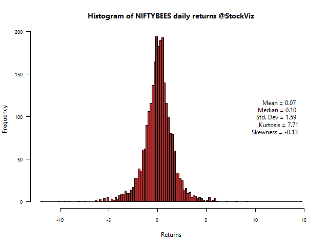
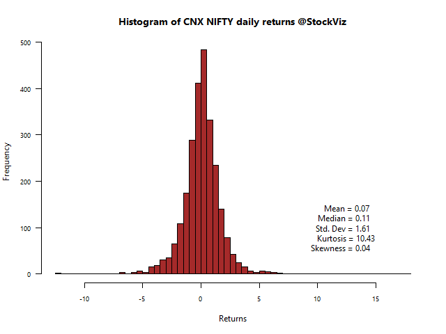
But returns, on the other hand, are distributed somewhat like a normal (Gaussian) distribution.

nifty-histogram

And there doesn’t seem to be any auto-correlation between consecutive returns.

nifty-autocorrelation

If returns are normally distributed, then how are prices distributed? It turns out that the logarithm of the price is normally distributed. Why? Because

returns(t) = log(price(t)/price(t-1))

Now statisticians can magically transform a random time-series (prices) into something that is normally distributed (returns) and work with that instead. Almost all asset pricing models that you will come across in literature has this basic assumption at heart.

Fat tails

The assumption that returns are normally distributed allow mathematically precise models to be constructed. However, they are not very accurate.

In the normal distribution, events that deviate from the mean by five or more standard deviations (“5-sigma events”) have lower probability, thus meaning that in the normal distribution rare events can happen but are likely to be more mild in comparison to fat-tailed distributions. On the other hand, fat-tailed distributions have “undefined sigma” (more technically, the variance is not bounded).

For example, the Black–Scholes model of option pricing is based on a normal distribution. If the distribution is actually a fat-tailed one, then the model will under-price options that are far out of the money, since a 5- or 7-sigma event is much more likely than the normal distribution would predict.

Precision vs Accuracy

When you build models, the precision that they provide may lull you into a false sense of security. You maybe able to compute risk right down to the 8th decimal point. However, it is important to remember that the assumptions on which these models are build don’t led themselves to accuracy. At best, these models are guides to good behavior, and nothing more.

accuracy vs precision

Sources:
Fat-tailed distribution

Analysis: Bhavin Desai’s Bull Spread on ITC

Bhavin Desai of Motilal Oswal Securities was on CNBC saying that one may buy ITC 350 Call and advises shorting 360 Call. This is a 350/360 long call spread on ITC. Let’s see how the trade works.

The greeks

ITC Bull Spread Greeks

The 360 call has a θ of -145.36 and it the model premium is 3.04. This means that the time decay will make the option worthless in a couple of days. Not bad since you are an option seller.

The 350 call is already ITM (the stock closed at 352.70) and the last traded price, Rs. 6.3 is less than the model price of Rs. 7.49. Not a bad deal.

Payoff diagram at expiry

ITC Bull Spread P&L

ITC Bull Spread Breakevens


ITC needs to be above Rs. 354.35 at expiry for this trade to break-even. Max loss is the premium paid upfront (Rs. 4350)

The right trade for the wrong reasons?

The transcript on moneycontrol says:

ITC has had some amount of shorts right from the beginning of this expiry and since then it has not done anything and once again since yesterday’s trade we have been seeing some amount of long additions. So, a call spread or rather a bull call spread is something that can be advised.

We are not really sure what that means. The reason why you would put a bull spread on is if you are moderately bullish about the stock and want to mitigate the cost of buying the lower strike by selling a higher strike.

Reference

Buy ITC 350 Call, short 360 Call: Bhavin Desai

Options Liquidity

Liquidity (or the lack thereof)

Open interest is a measure of liquidity of a particular market. For each buyer of a contract there must be a seller. From the time the buyer or seller opens the contract until the counter-party closes it, that contract is considered ‘open’. OI refers to the total number of derivative contracts that have not been settled.

Other than a few select indices and stocks, there is absolutely no liquidity in the option market. Here’s a chart of the latest total OI for the nearest (April) expiry:

OI April

And its worse for the next series:

OI May

Bid-offer spread

The problem with trading illiquid options is that the bid-offer spread ends up killing your trade. Compare and contrast the spreads for UNITECH and DABUR:

UNITECH APRIL

UNITECH MAY

DABUR APR

DABUR MAY

Don’t stop at trade setups

When you conceive option trades, make sure you consider liquidity constraints. Otherwise, your trade is likely to remain on paper.

The liquidity footprint is not static. For example, RCOM, which was #8 in Jan is nowhere to be found in the liquid dozen in April:

OI Jan

Monitoring liquidity risk is as important as checking your deltas and P&L and can often make or break a trade.