Tag: backtest

VIX and Equity Index Returns, Part I

shyam November 12, 2018November 13, 2018

The VIX is a measure of implied volatility of the underlying index. For example, the CBOE Volatility Index is a measure of 30-day expected volatility derived from S&P 500 Index call and put option prices, India VIX similarly uses the NIFTY 50 call and put options prices to derive a measure of volatility. The question we will try to address in this series of posts is whether the VIX can be used to time entries and exits on the underlying index.

The VIX time-series

The VIX on S&P 500 has been around since the 90’s whereas India VIX started out around 2009. Moreover, the US enjoys a much wider and deeper market for volatility products than any other market in the world. VIX futures, VIX options, VIX of VIX, volatility ETFs and their inverse, all trade fairly well. Whereas in India, even though VIX futures have been listed for a while, it rarely trades. Trading activity of a derivative (VIX, in this case) invariably has an effect on the underlying (S&P 500, NIFTY 50…) So we expect the relationship between S&P 500 VIX and the S&P 500 index to be closer than that between India VIX and the NIFTY 50 index.

VIX quintiles

To begin, we will bucket the trailing 1000-day VIX closing prices into quintiles and observe the next 5, 10, 15 and 20-day returns of the underlying index over them.
S&P 500 VIX

And, more recently:

What is striking here, is that subsequent returns off the 5th quintile (when VIX is at its highest) is higher with smaller negative outliers than returns off the 1st quintile (when VIX is a its lowest.) This is counter-intuitive to the notion that “volatility begets volatility” so investors are better off staying away from the market when it is volatile.

India VIX and NIFTY 50 shows a similar pattern*:

*Smaller sample compared to the S&P 500 dataset.

A simple back-test

What happens to a long-only portfolio if it is long the index only when the VIX is within a particular quintile?
S&P 500/VIX

The strategy that is long when VIX is in the 5th quintile (L5) out-performs the other quintile strategies. Also, if you ignore the 2008 collapse, L5 has the shallowest of drawdowns.
NIFTY 50/VIX
Something similar happens with NIFTY 50 as well:

Implications

Cash-only investors can point to the superiority of buy&hold compared to these VIX-based strategies. However, the shallow drawdowns exhibited by the L5 strategy (long index when VIX is in the 5th quintile) is attractive to leveraged traders. For example, NIFTY 50 futures leverage is between 8x and 10x. So even if you play it safe and leverage only 5x, L5 returns would end up at ~100% compared to buy&hold’s 80% over the same period.

We will dig deeper in the next part of this series. Stay tuned!

Code and more charts are on github.

Categories Investing Insight Tags backtest, VIX, volatility

Timing Entries and Exits based on Profits and Drawdowns

shyam October 25, 2018

We previously looked at a couple of popular “buy the dip” strategies – one based on SMA crosses and another based on drawdowns – and showed how they underperform a systematic daily SIP. Further, we showed how a daily SIP is not that different from a monthly SIP here. These studies were based on maximizing the terminal asset size. i.e., a strategy was labeled superior if it accumulated the maximum number of units of an index, mutual fund or stock. They weren’t trading strategies trying to maximize profits but investment strategies looking to maximize assets. Here, we turn our gaze to a strategy that lies in between investment and trading – exiting based on profit-booking and re-entering.

Book profits and re-enter

We often hear media pundits asking their followers to “book profits and re-enter at a lower level.” We wanted to see if it can be quantified systematically. What exactly does it mean in numbers? Is it better than buy and hold? So, we setup a backtest:

Start with a long
Once the long reaches a profit threshold, exit.
Stay out of the market until a drawdown point has been reached and then re-enter.
Do this for NIFTY 50, MIDCAP 100 and SMLCAP 100 indices.

Results

The tables below collate returns for 10-year rolling windows.

‘BH’ indicates buy&hold.
‘RET_SEN’ and ‘RET_MAX’ are the scenarios that produce the best returns, respectively.
‘IR_SEN’ and ‘RET_IR’ are the scenarios that produce the best information ratio and its corresponding returns, respectively.

As you can see, there is no clear winner here. However, there are some configurations that seem to repeat. For NIFTY 50, it appears to be 35%:10% i.e., sell once returns have reached 35%, re-enter on a 10% correction. For MIDCAP, you could probably go with 70%:10% and for SMLCAP, 80%:15%. Below are their respective cumulative and yearly return charts:

NIFTY 50

MIDCAP 100

SMLCAP 100

Applying the strategy to MIDCAP and SMLCAP seem to have some merit. However, when you look at the yearly returns chart, it is obvious that a bulk of the out-performance came from just two or three years of the ~20 year dataset. Another key observation here is that these strategies do not offer any significant downside protection. Also, these back-tests do not incorporate the tax impact and transaction costs of these strategies.

Takeaway

“Book profits and re-enter at a lower level” may sound like a nice thing to do but there is no consistent rule that can be applied that can justify the added costs and tax impact.

Code and more charts on github.

Categories Investing Insight Tags backtest

Is Skewness a Timing Signal?

shyam October 19, 2018

We recently came across a post titled “IMPROVING THE ODDS OF VALUE” (link,) where the author uses the skewness of one-year daily returns to time the value factor. Here, we try to replicate/extend the original backtest.

Key differences

We had to make some tweaks to simplify the task:

The original uses a one-year lookback period, we use a 220-day (trading days) lookback. [minor]
The original uses the S&P 500 index, we use the SPY ETF. Our prices are adjusted for dividends. [minor]
The original constructs a long-short value portfolio. i.e., an academic alpha portfolio. We use it to time the IVE ETF which tracks the S&P 500 Value Index. [major]

We expected the major premise of the original post – that you can go long value during periods of positive skewness and go into cash otherwise – to hold. And perhaps provide some marginal advantage while using it to time a long-only value ETF.

Results

We observed the exact opposite result. Going long IVE during periods of positive skewness under-performed going long IVE during periods of negative skewness. In the cumulative returns chart below:

the black and red lines are buy&hold IVE and SPY,
the green and blue lines are IVE returns when being long during periods of positive and negative skewness, respectively,
the cyan and purple lines are SPY returns when being long during periods of positive and negative skewness, respectively,

Note how buy&hold vastly out-performs the timing portfolio.

Further, if you rotate into a liquid fund (earning risk-free returns) instead of going into cash (earning zero), the SPY returns being long during periods of negative skewness beat buy&hold SPY returns:

Perhaps, we are seeing these totally different results because we are long-only and the original back-test was long-short? We are not entirely sure.
Also, the out-performance we observed on SPY failed to replicate on the NIFTY 50 and NIFTY MIDCAP 100 indices.

Code, charts and backtest results for NIFTY 50 and NIFTY MIDCAP 100 indices are on github.

Categories Investing Insight Tags backtest, quant

Simple Momentum with Transaction costs and Taxes

shyam July 13, 2018

The earlier post on a simple momentum strategy ignored transaction costs and taxes. Typically, these are added to backtests where gross profits are high enough to consider them for further analysis. However, one of readers requested that we add these costs to get an idea of their effect on returns.

To keep things simple, we assumed a 25bps net transaction cost and a 10% tax on gains. The tax part is a bit tricky so we ran the analysis with some simplifying assumptions. Follow the github link to the code if you are curious.

Running with these assumptions, transaction costs and taxes lopped 82% off gross returns over Jan 2005 through June 2018.

What kills you are the taxes, not the transaction costs. There were only 17 trades throughout the period. It is the 10% tax on gains that ruins the compounding.

Code and other charts are on github. Look for ones with a ‘tx’ in the suffix.

Categories Investing Insight Tags backtest, momentum

Simple Momentum

shyam July 11, 2018

Michael Batnick, in his blog titled “Simple Momentum,” proposes a strategy that follows a simple rule:

If the S&P 500 outperformed 5-year U.S. treasury notes over the previous twelve months, invest 100% of this portfolio in the S&P 500 in the following month. If the 5-year U.S. treasury notes outperformed the S&P 500 over the previous twelve months, invest 100% of this portfolio in bonds in the following month.

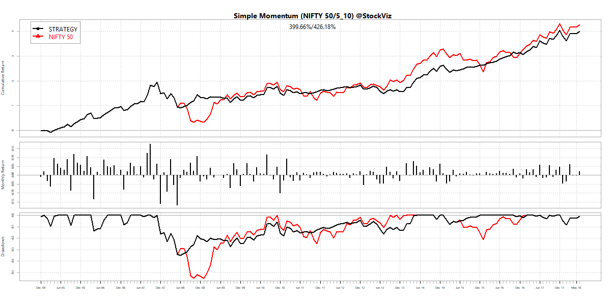
It outperformed the S&P 500 with significantly lower drawdowns. Could the same strategy work with Indian indices? We took NIFTY 50 and MIDCAP 100 indices and paired it with the 5-10 year tenure gilts.

Returns

The strategy returns are significantly lower than a simple buy and hold. December 2004 through June 2018, the NIFTY 50 version of it under performed buy and hold by 6% and the MIDCAP 100 version by 34%. This is before transaction costs and taxes. Here are the cumulative return charts:

Drawdowns

The simple momentum strategy did have lower peak drawdowns than a buy and hold:

What keeps you out of the troughs also ends up keeping you out of the peaks. This is highlighted by how the strategy behaved in 2008 and 2009:

Conclusion

The simple momentum strategy is perhaps too simple. The backtest doesn’t capture transaction costs and taxes that would further ding the already lagging gross returns.

You can peruse the code and the charts used in this blog on github.

Categories Investing Insight Tags backtest, momentum