Tag: macro

Please read Part I and Part II for an introduction.

In Parts I and II, we saw how a polynomial kernel was probably a good way to tune an SVM. Also, there was no single degree parameter that was necessarily better than the others. In this post, we train three different polynomial kernel SVMs on two other dollar indices (DTWEXB and DTWEXO) and USDINR (DEXINUS) and tabulate their returns over the two different datasets and across different degree parameters.

To recap, The FRED publishes the following indices along with USDINR (DEXINUS):

1. DTWEXB: Trade Weighted U.S. Dollar Index: Broad
2. DTWEXM: Trade Weighted U.S. Dollar Index: Major Currencies
3. DTWEXO: Trade Weighted U.S. Dollar Index: Other Important Trading Partners

We modeled DTWEXM in Parts I and II. Here, we model the rest.

Results

2000-2018

2005-2018

Given the results above, we can ignore DTWEXO going forward. Surprisingly, DEXINUS (USDINR) does not predict the 2018 correction. In fact, the DEXINUS model using the 2005-2018 dataset replicates buy&hold. Hence, we will ignore DEXINUS as well. The SVM modeled on the 2005-2008 dataset using DTWEXB with degrees 5, 6 and 8 seem to have side-stepped the 2016 and 2018 corrections. Furthermore, degree 8 seems to have produced the best cumulative returns on the test set.

Next steps

Our observation from Part II was that a 2005-2018 dataset is probably a better set than 2000-2018. This is confirmed from the DTWEXB model above. In the next post, we will combine the DTWEXB(8) and DTWEXM(4) SVM models using the 2005-2018 datasets.

Code and charts are on github.

Please read Part I for an introduction.

Earlier, we saw that a 3rd degree polynomial kernel produced the best results on the test set. In this post, we explore if we can we get better results by tuning the degree parameter.

Outline

1. Use 1-, 2-, 5- and 10-week returns of DTWEXM to train an SVM using a polynomial kernel on subsequent 1-week returns of the NIFTY 50
2. Consider two datasets: one between the years 2000 and 2018 and the other between 2005 and 2018
3. Divide the dataset into training/validation/test sets in a 60/20/20 ratio
4. Use the validation test to tabulate out-performing degree parameters
5. Plot the cumulative return of a long-only, long-short and buy&hold NIFTY 50 strategy based on SVM predictions on the test set

Results

We find that there is no single degree parameter between the two datasets (#2 above) that consistently outperforms.

2000-2018 dataset

2005-2018 dataset

Here are the cumulative return charts for the best performing parameter:
2000-2018 dataset (8)

2005-2018 dataset (4)

While the first model (using the 2000-2018 dataset, 8th degree polynomial) failed to “predict” the 2018 correction in the NIFTY 50, the second one (2005-2018 dataset, 4th degree polynomial) seems to be able to side-step it. However, an SVM tuned with the 4th degree polynomial on the 2000-2018 dataset again failed to side-step the 2018 correction, indicating that we need to look more closely on how we choose our dataset – sometimes going too far back in time is counter-productive because the world changes.

Next Steps

In the next post, we will train a polynomial SVM with the other dollar indices (DTWEXB and DTWEXO) and USDINR (DEXINUS) and tabulate their predicted returns over different degrees.

Code and charts for this post are on github.

This series of posts pulls together two things we observed in our previous posts:

1. There is a non-linear relationship between USDINR and the NIFTY (NIFTY vs. INR/OIL Correlation)
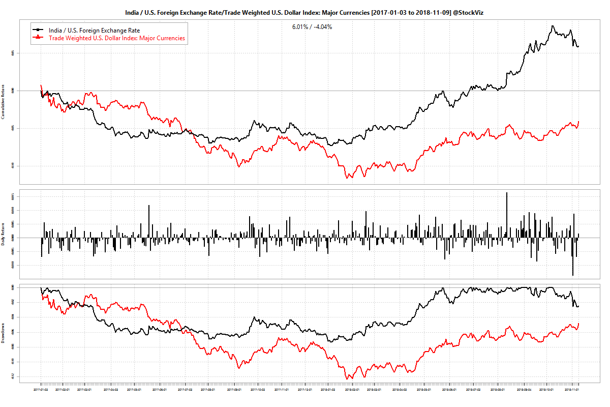
2. There is a stable spread between USDINR and currency indices published by the FRED (USDINR and Dollar Indices)

Here, we use a Support Vector Machine (SVM) to train a model on the returns between the DTWEXM index (Trade Weighted U.S. Dollar Index: Major Currencies) and the NIFTY 50.

Outline

1. Use 1-, 2-, 5- and 10-week returns of DTWEXM to train an SVM on subsequent 1-week returns of the NIFTY 50
2. Consider two datasets: one between the years 2000 and 2018 and the other between 2005 and 2018 to include/exclude the 2008 market dislocation
3. Divide the dataset into training/validation/test sets in a 60/20/20 ratio
4. Use the validation test to figure out which SVM kernel to use
5. Plot the cumulative return of a long-only, long-short and buy&hold NIFTY 50 strategy based on SVM predictions on the test set
6. Use the common kernel between the #2 datasets for future experiments

Results

We find that an SVM using a 3rd degree (the default) polynomial kernel gives the “best” results. We use the SVM thus trained to predict next week NIFTY returns and construct long-only and long-short portfolios.

Here are the cumulative returns when the dataset considered is the one between 2000 and 2018. The test set runs from 2015 through 2018:

There are some points of concern. For one, the model is heavily long-biased. Even when the actual returns were negative, the predicted values was mostly positive:

Second, the model has tracked the buy&hold NIFTY since the beginning of 2018. The narrative has been that the rise in oil prices caused the CAD to blow out that caused investors to pull out investments that caused the rupee and NIFTY to fall (whew!) Either USDINR moved independently of DTWEXM or the relationship between DTWEXM and NIFTY 50 broke down. It looks like its the former:

Third, the cumulative returns seem to have been majorly influenced by small set of predictions that cut a drawdown that occurred in July-2015 by half. We notice a similar effect on the smaller dataset (2005 through 2018):

See how a small branch in Nov-2016 lead to the superior returns of the model predicted portfolios.

Next steps

In the next part, we will fiddle around with the degree of the polynomial used in the kernel to see if it leads to better returns. Subsequent posts will cover the use of the other dollar indices (DTWEXB and DTWEXO) and finally USDINR (DEXINUS) itself.

Code and charts for this post are on github