Tag: lumpsum

This is a continuation of Lumpsum vs. Dollar Cost Averaging (SIP) that modeled different return series and concluded that a prudent investor would be better off with a SIP because of a smaller probability of incurring a large loss. However, we stopped short of comparing different indexes to see if the conclusion held.

The ‘average’ return

What happens if we take the average weekly return of an index and create a synthetic index that just gives those average returns without any variance? We end up with a parabolic looking cumulative return profile below:

The small cap index was chosen on purpose to illustrate how ‘average’ returns relate to real returns on an extremely volatile index.

The average return series is, of course, a fantasy. What we are interested in is in the probability of getting those returns.

Probabilities

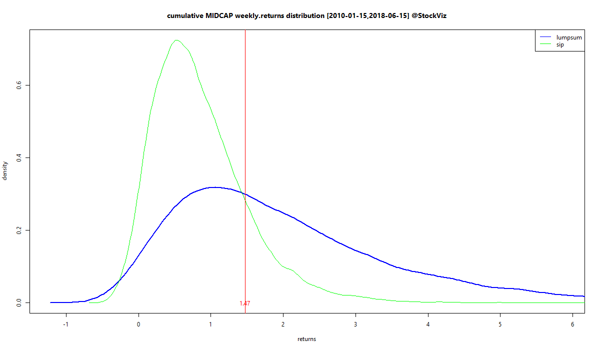
Just like our first post, we start by modeling the returns of the NIFTY 50, MIDCAP and SMLCAP indexes as a Generalised Lambda Distribution and running a 10,000 path simulation to obtain a series of DCA vs lumpsum investment returns. We then feed that into a empirical cumulative distribution function so that we can query it for probabilities under different thresholds. To put that in a picture:

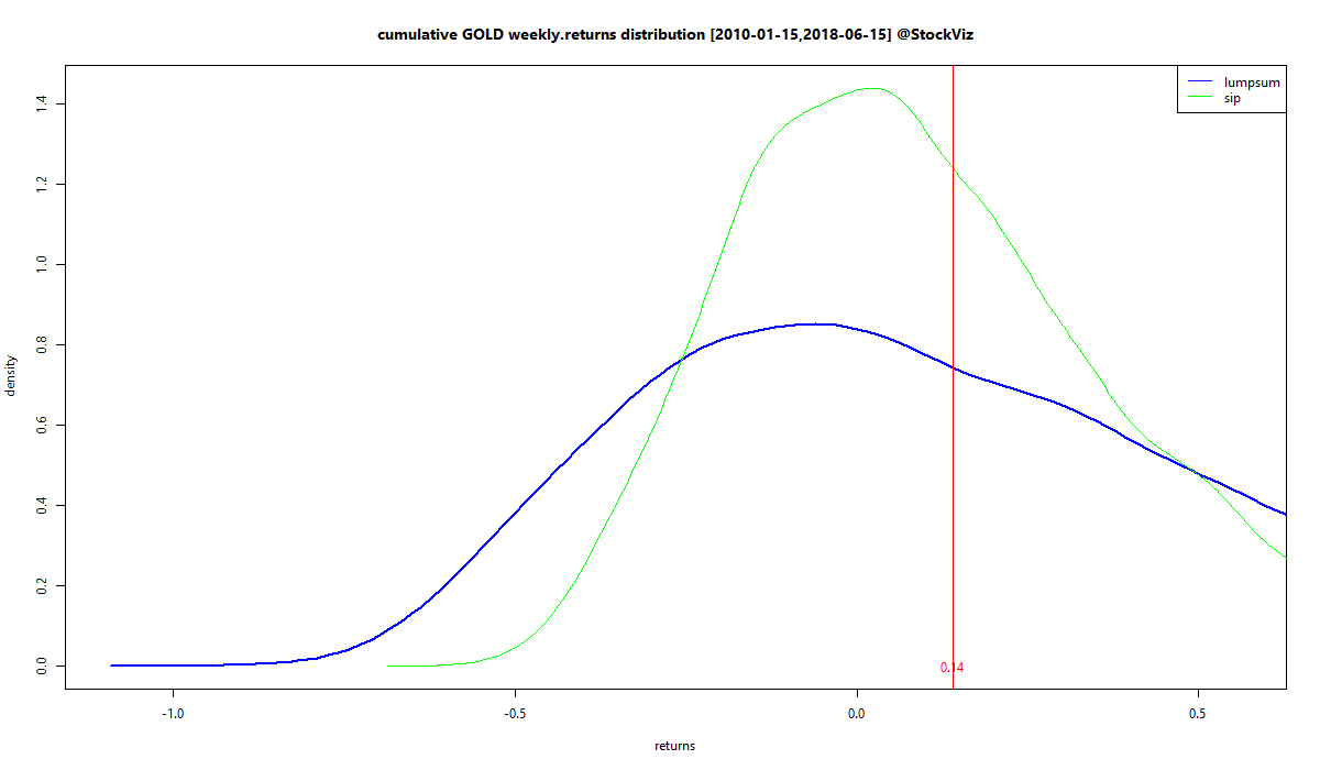
The vertical lines mark the different thresholds we are interested in.

• The grey line on the left is at zero. We have SIP showing a 4.44% probability of negative returns and lumpsum showing 3.49%. Yes, there is a non-trivial possibility that SIPs will give negative returns. However, looking at the shapes below zero, SIP losses may not be as large as lumpsum losses.
• The red line in the middle is the start to finish return of the index. Here, we have SIP showing a 22.69% probability of exceeding those point-to-point returns and lumpsum showing 57.50%.
• The orange line on the right is the compounded ‘average’ return. We have SIP showing a 7.82% probability of exceeding that and lumpsum showing 37.20%.

Here is the same MIDCAP:

And for NIFTY 50:

What does all this mean?

1. It is possible for SIP returns to be negative over large periods of time. Enough to cover your entire investing lifetime. So, if you are investing in small-caps, make sure you are not 100% allocated to it.
2. Lumpsum investing gives you a higher probability of higher returns across all indexes. The probability of negative returns are on par with that of SIP’s.
3. Lumpsums have fatter left tails. However, if you are looking only at NIFTY 50 and MIDCAP, those probabilities are tiny.
4. Lumpsums have a higher probability of achieving ‘average’ returns compared to SIPs.
5. Lumpsums seem to be benefiting from “time in the market” on indexes that rise over a period of time.

Code and charts on github.

Among Indian investors, SIPs (Systematic Investment Plans) are the rage right now. The total amount collected through SIP during May 2018 was ₹7,304 crore according to AMFI. SIPs are great for investors with a regular income – it matches the frequency of savings with the frequency of income. Structural discipline is always a welcome thing. However, for investors who have lumpy incomes or a windfall, it is often a dilemma whether to invest as a lumpsum or to setup an STP (Systematic Transfer Plan.)

Both SIPs and STPs are a form of DCA (Dollar Cost Averaging) where you average into an investment over a period of time (the accumulation phase.) The thing about DCA is that it ends up under-performing a lumpsum in markets that are trending up. Intuitively, you want to buy more when the price is low (in the beginning) and less when the price is high (at the end.) So, if the market is going up, then it makes no sense to spread a lumpsum over a period of time – you are guaranteed to make the later buys at a higher level, reducing your overall returns.

In the case of equity markets, the expectation is that they tend to go up over time. So if you are looking at a 10-20 year time horizon, then you are better off investing in one shot. To put this intuition to test, we modeled the returns of NIFTY, MIDCAP and GOLD as a Generalised Lambda Distribution (this works better than a normal distribution because these returns have significant skews and kurtosis) and ran a 10,000 path simulation to get a sense of the probability distribution of DCA vs lumpsum investments.

Roughly, this is like assuming that the weekly return distribution is going to be the same across 10,000 different worlds. So you pick set of random weekly returns from the same distribution 10,000 different times and see how DCA and lumpsum perform over those worlds. When you plot the density of those returns, you get an idea of how they compare.

To keep things simple, lets compare NIFTY MIDCAP 100 and GOLD. First, the price charts:

And now the simlulated cumulative return densities of MIDCAP and GOLD, modeled with data after 2010:

The area to the left of zero is that of negative returns. Lumpsums have a longer left tail compared to DCA so probability of a large negative outcome is higher for the former.
However, the total area under zero is higher for DCA in MIDCAPs so the probability of negative outcomes in general is higher for DCA/SIP.
Lumpsums have a fat right tail for both MIDCAPs and GOLD so the probability of large positive outcomes is higher for lumpsums.
“Average” DCA returns are less than “average” lumpsum returns but they occur with a higher probability.

For a prudent investor, it is the left tail that matters the most. Even though lumpsums hold out hope for higher returns (fat right tails,) they have a small probability of a big loss that is greater than that for DCA (longer left tails.) In conclusion, a prudent investor should convert a windfall into an STP and a risk-seeker should do a lumpsum.

For readers curious about the code and for additional charts with longer time periods, visit github.