The book Trading and Exchanges (Amazon,) has a section on Roll’s Serial Covariance Spread Estimator which tackles the problem of estimating the bid/ask spread with only the price series.
The Roll’s serial covariance spread estimator is an econometric model designed to estimate the average bid/ask spread (or effective spread) of a security using only transaction prices, without needing quotation data. It is one of the best-known estimators based on price change serial covariances.
The idea is from the 90’s and we’ve come a long way since then. Now, we have streaming quotes from which the spread can be directly computed. What makes this approach interesting is the decomposition of volatility that was used to estimate the spread can be used to estimate fundamental volatility instead.
Total Volatility = Fundamental Volatility + Transitory Volatility
Fundamental volatility consists of seemingly random price changes that do not revert. These changes often have the properties of a random walk.
Transitory volatility consists of price changes that ultimately revert. This price reversal creates negative serial correlation in the series of price changes.
Using Roll’s model, Fundamental Volatility = Total Volatility – (Effective Spread)2/4
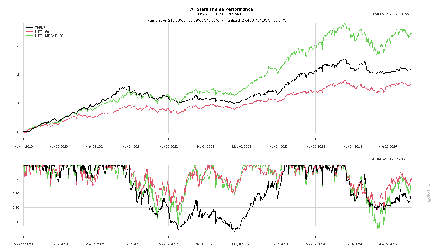
Here’s NIFTY through Roll’s model:

Code on Github.