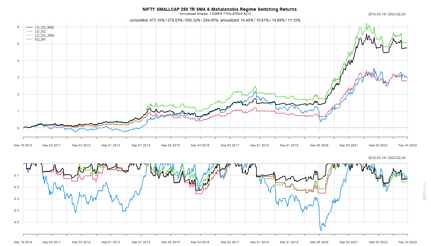
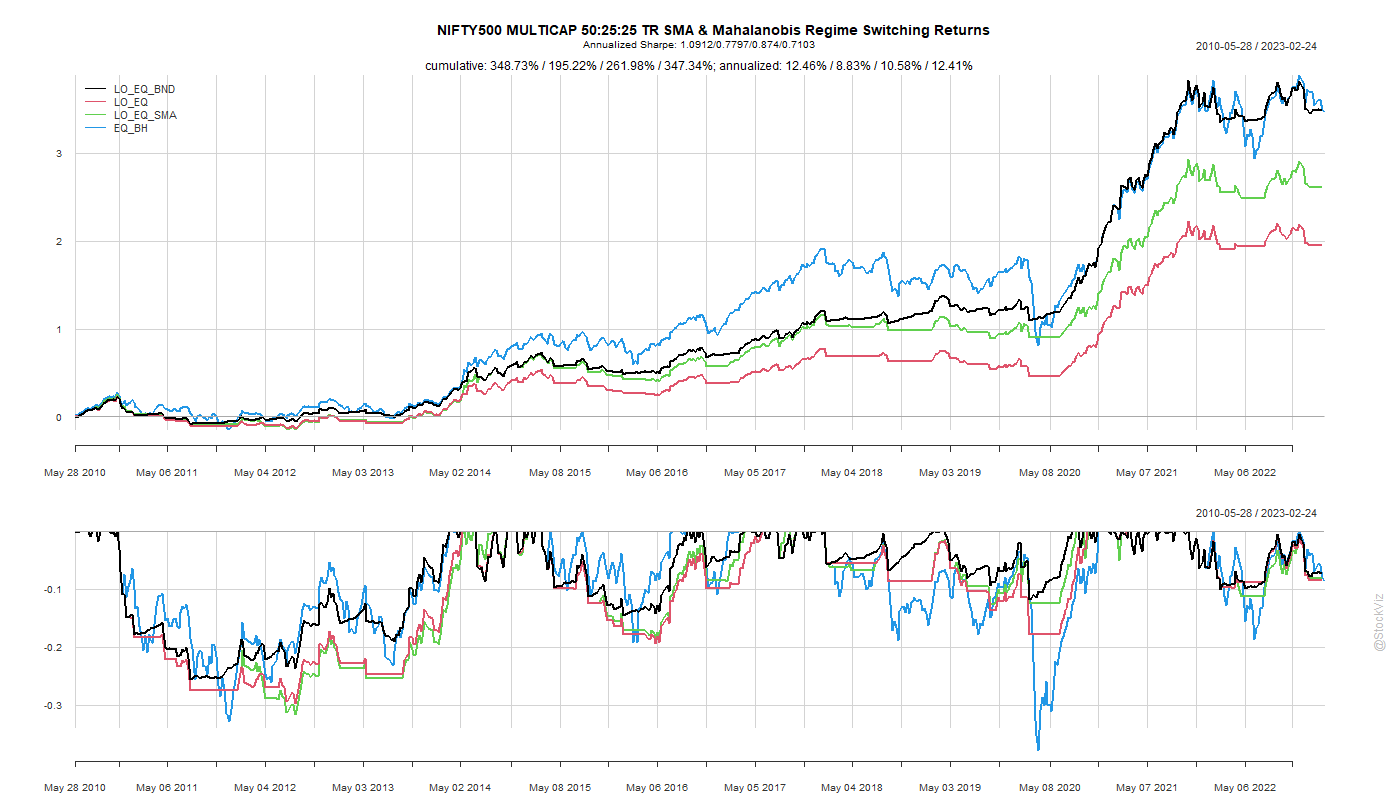
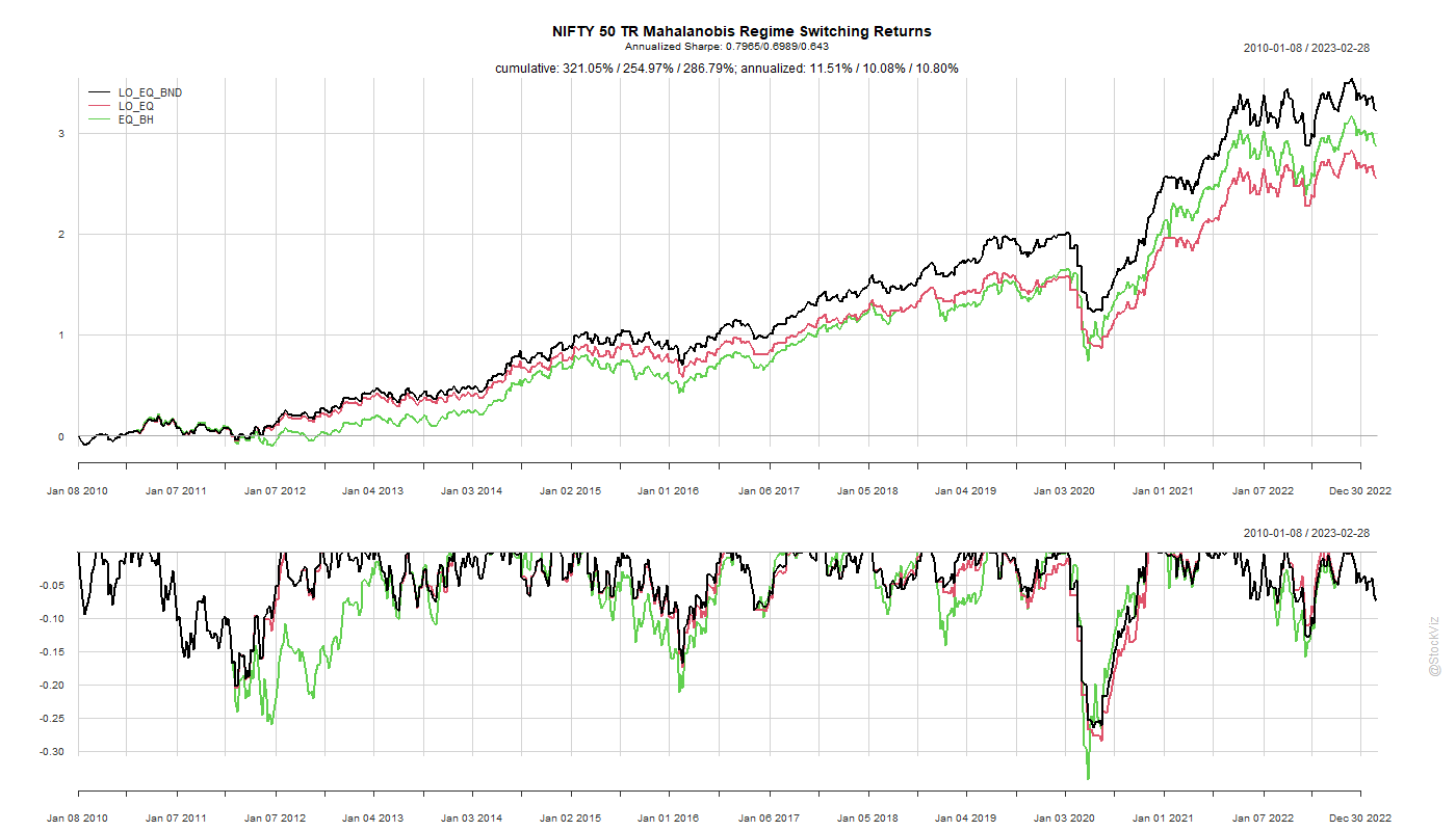
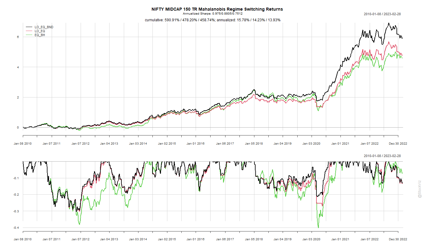
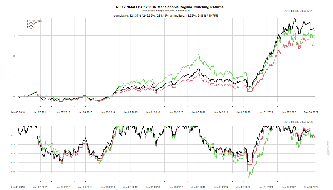
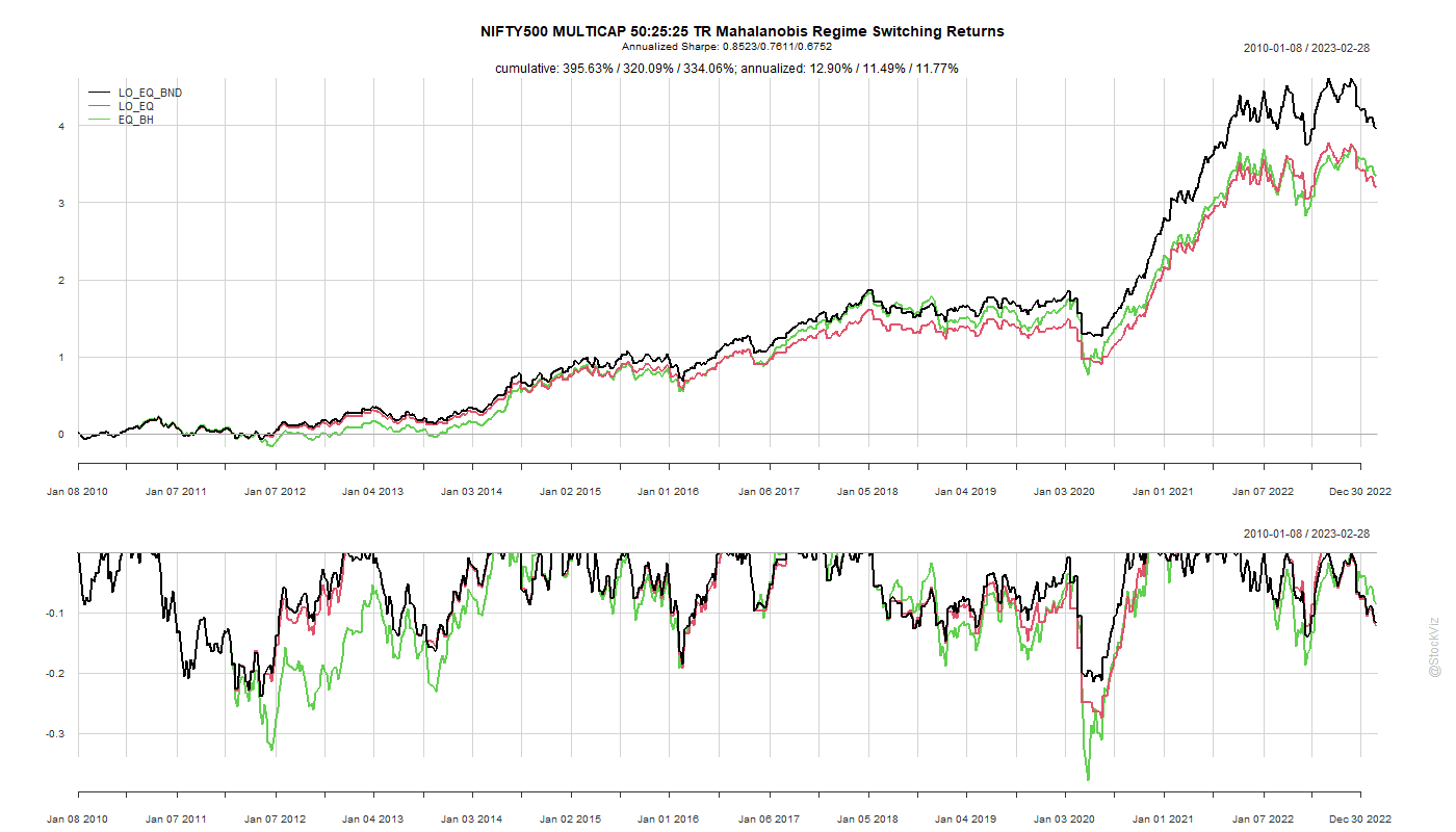
Recently, we came across an interesting paper, Skulls, Financial Turbulence, and Risk Management, Mark Kritzman, CFA, and Yuanzhen Li, that uses the Mahalanobis distance to construct a turbulence index. The basic idea is that the more asset returns break from the past, the more “significant” a market event.
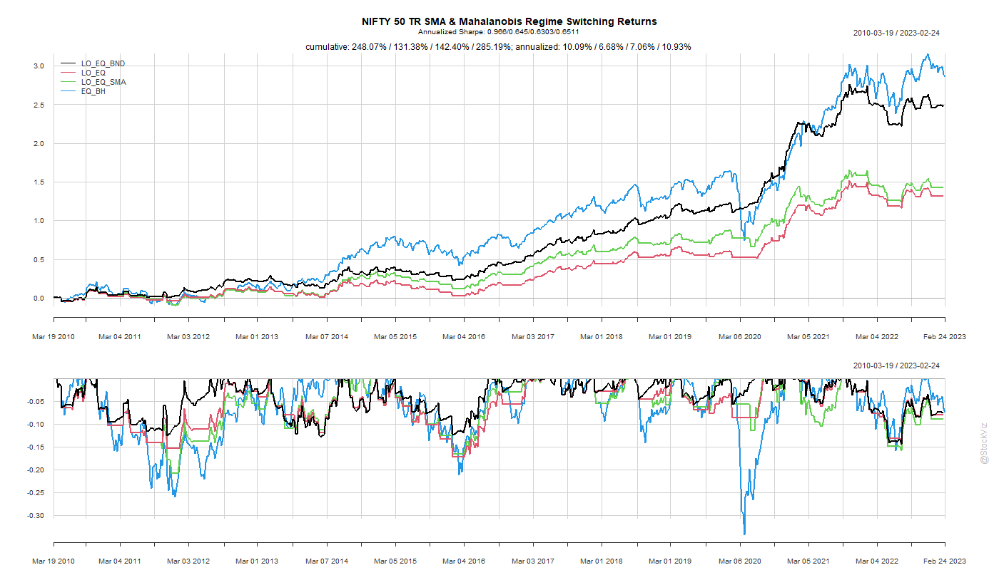
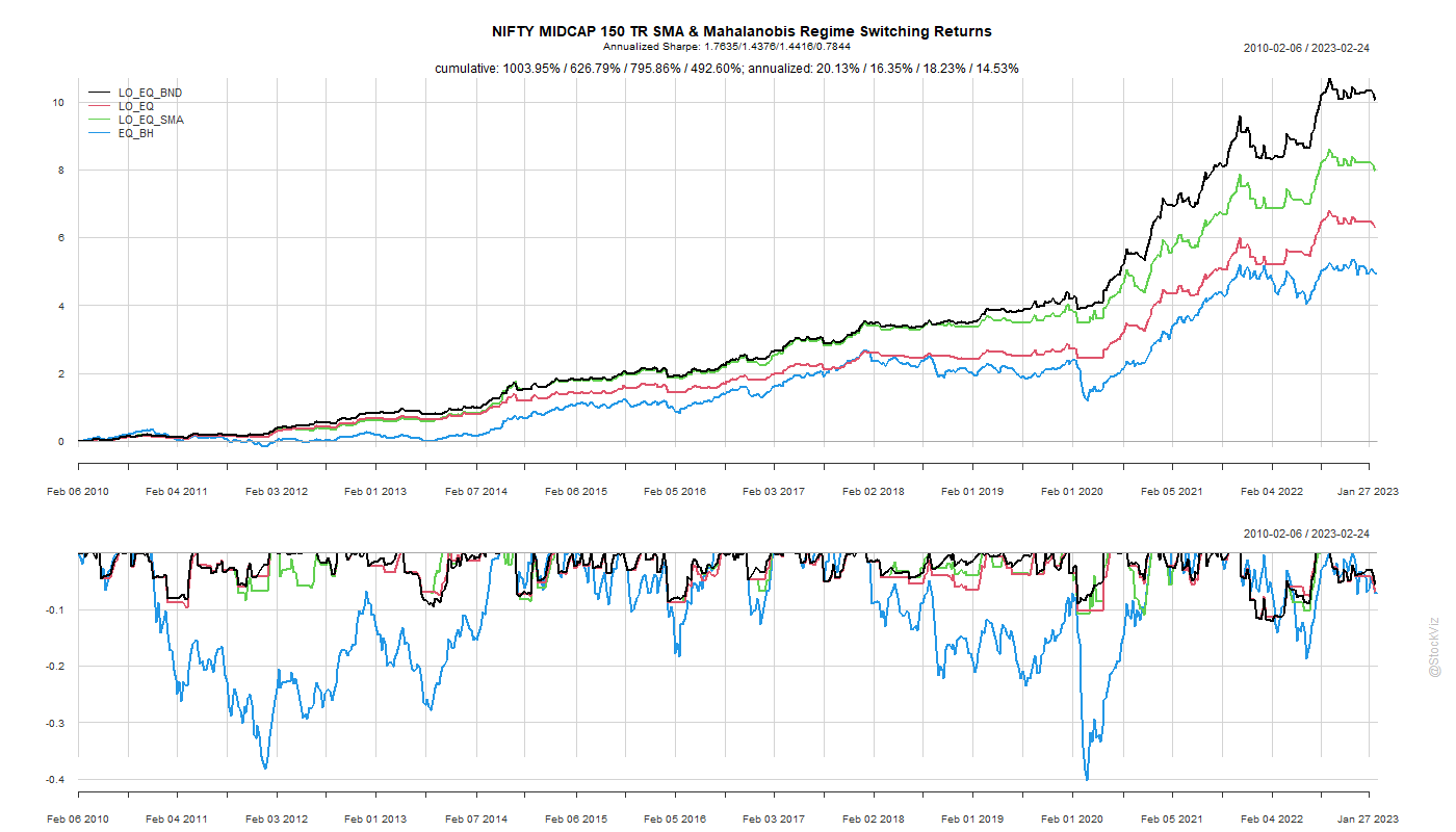
We took the basic intuition behind this and constructed a portfolio that switches between equities and bonds based on the Mahalanobis distance between them.
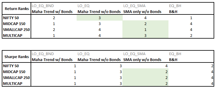
The out-of-sample results, factoring in transaction costs, look promising but doesn’t really stand out compared to other, more dumber, strategies that avoid steep drawdowns. However, two points over the Midcap buy & hold cannot be dismissed outright.
Hypothesis: If a price segment is similar to a set of historical segments, then there should be a correlation between historical and future returns.
Setup: Take 60-minute segments of 1-minute bars. Match them with 200 of the most recent days’ with times aligned. Take the top 40 days with the closest match and calculate their median next 30-minute returns. Plot the median vs. actual.
Simplifications:
Non-overlapping segments. Its can be argued that patterns don’t start and stop and perfectly aligned boundaries.
Most-recent 200 day look-back period. What if that’s not enough? Or too much?
Our previous post showed how a chrono-clock frequency can be translated into a volume-clock frequency. The aggregated High-Low price data looks very similar to a candle-stick chart.
The difference between the high and the low on each “candle” of the longest living contract doesn’t vary a lot between the two clocks.
The distribution is based on a month’s worth of streaming data. As we accumulate more data points, it is likely that the divergence between the Chrono-Clock and the Volume-Clock increases.
In our brief intro to the volume clock, we showed how you use a volume based aggregation to match the sampling frequency with information flow frequency. To further expand on that intuition, lets say that as a trader, you are used to watch the 5-minute chart. However, when markets turn volatile, you reach for the 1-minute or sometimes even the 30-second chart. Why is that?
In liquid futures markets like the NIFTY, volatility is associated with increased volume. A 5-minute window captures quite a wide range of volume.
While, on average, 10000 contracts get traded in a 5-minute interval, there are times when the market goes “berserk.” This is where the volume-clock begins to make sense. If you fix the volume at 10000, then your aggregation automatically tracks information flow without you having to zoom in and out.
Notice how the width of the window automatically expands and shrinks?
You can choose the volume interval to aggregate based on the current clock frequency that you use to trade.
Typically, prices and volumes are charted based on time aggregations. The most common aggregation is the daily chart.
The daily chart shows the high/low/open/close and volume traded of a particular instrument. Intraday traders might prefer a more granular version of this. Maybe a minute chart does the trick for them.
Chrono-clocks are intuitive because that’s how we perceive events around us and have been trained to think.
However, time is not the only way to aggregate prices. If prices are information, then volume indicates the speed with which it arrives. You can divide the day into equal volume buckets (eg. in 5000 contract increments) and transform the time-series from chrono-time to event-based time.
In fact, working in volume time presents significant statistical advantages. First, this time transformation removes most intra-session seasonal effects; second, it allows a partial recovery of Normality and the IID assumption; third, sampling in a volume-clock metric addresses the problem of random and asynchronous transactions, which is a major concern when computing correlations on high-frequency data.
The Volume Clock: Insights into the High Frequency Paradigm (SSRN)
We know that trading turnover throughout the day is not constant. If you plot turnover over a trading day, it typically traces a āUā shaped plot. Even widely traded index futures like the NIFTY have “slow” and “fast” periods. A volume clock is one way to match the sampling frequency with information flow frequency.
When you aggregate by volume, each slice of time will have different lengths. For example, we streamed NIFTY futures over a couple of weeks and aggregated it by 2500, 5000 & 10000 lots traded. The y-axis is the width of the time-slice of each volume-tick.
The size of the volume bucket would depend on what one is trying to analyze. Here’s the 2500 lot bucket by itself:
“There are minutes where nothing happens; and there are seconds where minutes happen” – Lenin, the High Frequency Trader.