Tag: backtest

Global Equities Momentum

shyam January 22, 2019

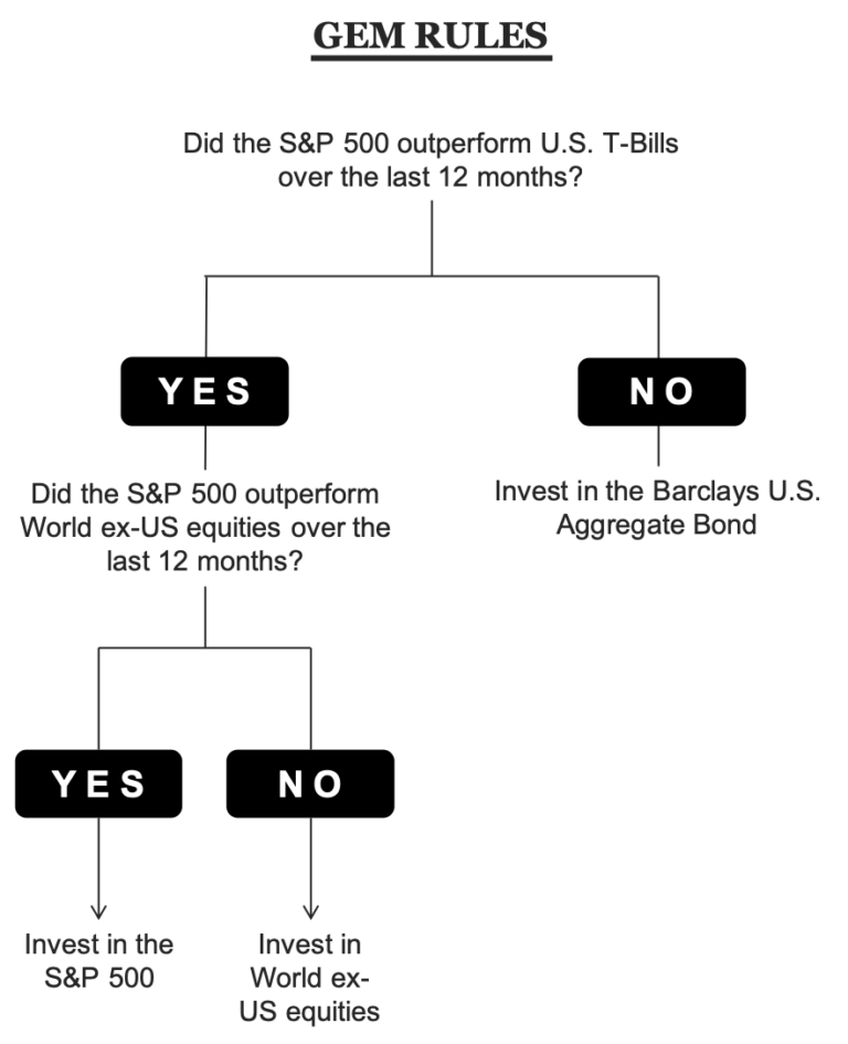
Gary Antonacci created the Global Equities Momentum (GEM) model that applied dual momentum to stock and bond indices. It toggles between stocks and bonds using 12-month trailing returns. And when it toggles to “stocks,” it chooses between US equities and International (ex-US) equities based on whichever posted higher returns in the previous 12-months. Newfound Research has a chart that puts it across succinctly:

The model uses the S&P 500 index as a stand-in for US equities and the WORLD ex USA index for international stocks. However, there is nothing in the construction that prevents us from replacing those market-cap based indices with momentum based ones.

US Momentum / Market-cap International

Scenario 1: keep everything the same, except in the last stage, instead of buying S&P 500, buy US Momentum (SP 500×1).
Scenario 2: swap out S&P 500 and put US Momentum everywhere in the decision tree (MOM).

In the cumulative return chart below, the black line is the base case. It represents GEM as originally designed. The red line is Scenario 1 above, green is Scenario 2.

Even though Scenario 2 has higher returns, it comes at the cost of higher drawdowns. Scenario 1 seems to strike a compromise.
Base case drawdowns:

Scenario 1 drawdowns:

Scenario 2 drawdowns:

US Momentum / International Momentum

What if, we bought International Momentum (WORLD ex USA MOMENTUM) instead of the market-cap based WORLD ex USA?
Scenario 3 (dark blue): keep everything the same, except in the last stage, instead of buying S&P 500, buy US Momentum. And instead of buying market-cap international, buy WORLD ex USA MOMENTUM (SP 500×2).
Scenario 4 (light blue): swap out S&P 500 and put US Momentum everywhere. And instead of buying market-cap international, buy WORLD ex USA MOMENTUM (MOMx2).

Scenario 3 drawdowns:

Scenario 4 drawdowns:

Here are returns broken down annually for all the scenarios discussed above:

It appears that using the S&P 500 index for making decisions about buying US vs. World ex-US momentum boosts returns while keeping a floor under drawdowns.

Code and charts are on github.

Categories Investing Insight Tags backtest, momentum

Streaks, Part II – Backtest

shyam January 3, 2019

In Part I of this series, we saw that it is very rare for two consecutive down months to be followed by a third one. Here, we present a simple backtest that goes long NIFTY 50 for a month if the previous two months were negative.

The shallow drawdowns of this strategy makes it ideal for leveraged trades. NIFTY futures are about 7x levered. That should transform the 190% gross return to about 1330%, beating buy and hold by a wide margin. The MIDCAP 100 index behaves similar to this between the 2005 through 2018 time-frame. However, the results are not so great if you include data prior to 2005.

This looks like a case of severe data-mining and should be discounted as such. But it is an interesting result nevertheless.

Code and charts are on github.

Categories Investing Insight Tags backtest, quant

SMA Distance, Part III – Backtest

shyam December 26, 2018

In Part II, we saw that when the 50- and 100-day SMA Distance is in the first quintile, subsequent 20-day returns have smaller left tails. Can that observation be turned into a market-timing system?

The backtest

We setup two long-only portfolios: one that goes long S&P 500 if either of the 50-day or 100-day SMA Distance is in the first quintile and another that, in addition to the 50- and 100-day being in the first quintile, also makes sure that the 200-day SMA Distance is not in the first quintile. These are L1 and L2 in the chart below:

Using SMA Distance is a poor long-term strategy. However, it does help avoid deep drawdowns. It is not very useful as a standalone indicator but perhaps could be used to confirm other signals.

Code and charts are on github.

Categories Investing Insight Tags backtest, sma

VIX and Equity Index Returns, Part II

shyam November 13, 2018

Please read Part I for the introduction.

Holding-period back-test

In Part I, we ran a quick back-test that would go long the equity index if the VIX was in a certain quintile and saw how the 5th quintile produced the lowest draw-down returns. The index was held only for a day. However, our box-plot of VIX quintile vs. subsequent n-day returns begs us to look at alternate holding periods as well. What would the returns be if we held onto the index beyond a day?

Here is how long-only S&P 500 returns when VIX is in the 5th quintile, across different holding periods looks like:

The problem with this strategy is that when there is a steep fall in the index, the VIX keeps going higher and will be in the 5th quintile for an extended period of time. Have a look at the 2008-2009 segment in this chart:

What happens if we used the change in VIX to time the equity index?

VIX returns deciles

If we bucket VIX returns (percentage change over previous close over n-days, 1000 trailing observations) into deciles and observe the next 5, 10, 15 and 20-day returns of the underlying index over them:

There is no determinable pattern here. Perhaps the VIX and the index are co-incident with none holding the power of prediction over the other.

Interested readers can browse the github repo for corresponding Nikkei 225 and NIFTY 50 charts.

Categories Investing Insight Tags backtest, VIX, volatility

VIX and Equity Index Returns, Part I

shyam November 12, 2018November 13, 2018

The VIX is a measure of implied volatility of the underlying index. For example, the CBOE Volatility Index is a measure of 30-day expected volatility derived from S&P 500 Index call and put option prices, India VIX similarly uses the NIFTY 50 call and put options prices to derive a measure of volatility. The question we will try to address in this series of posts is whether the VIX can be used to time entries and exits on the underlying index.

The VIX time-series

The VIX on S&P 500 has been around since the 90’s whereas India VIX started out around 2009. Moreover, the US enjoys a much wider and deeper market for volatility products than any other market in the world. VIX futures, VIX options, VIX of VIX, volatility ETFs and their inverse, all trade fairly well. Whereas in India, even though VIX futures have been listed for a while, it rarely trades. Trading activity of a derivative (VIX, in this case) invariably has an effect on the underlying (S&P 500, NIFTY 50…) So we expect the relationship between S&P 500 VIX and the S&P 500 index to be closer than that between India VIX and the NIFTY 50 index.

VIX quintiles

To begin, we will bucket the trailing 1000-day VIX closing prices into quintiles and observe the next 5, 10, 15 and 20-day returns of the underlying index over them.
S&P 500 VIX

And, more recently:

What is striking here, is that subsequent returns off the 5th quintile (when VIX is at its highest) is higher with smaller negative outliers than returns off the 1st quintile (when VIX is a its lowest.) This is counter-intuitive to the notion that “volatility begets volatility” so investors are better off staying away from the market when it is volatile.

India VIX and NIFTY 50 shows a similar pattern*:

*Smaller sample compared to the S&P 500 dataset.

A simple back-test

What happens to a long-only portfolio if it is long the index only when the VIX is within a particular quintile?
S&P 500/VIX

The strategy that is long when VIX is in the 5th quintile (L5) out-performs the other quintile strategies. Also, if you ignore the 2008 collapse, L5 has the shallowest of drawdowns.
NIFTY 50/VIX
Something similar happens with NIFTY 50 as well:

Implications

Cash-only investors can point to the superiority of buy&hold compared to these VIX-based strategies. However, the shallow drawdowns exhibited by the L5 strategy (long index when VIX is in the 5th quintile) is attractive to leveraged traders. For example, NIFTY 50 futures leverage is between 8x and 10x. So even if you play it safe and leverage only 5x, L5 returns would end up at ~100% compared to buy&hold’s 80% over the same period.

We will dig deeper in the next part of this series. Stay tuned!

Code and more charts are on github.

Categories Investing Insight Tags backtest, VIX, volatility