We are big fans on using distance measures while prospecting for investment strategies. Previously:
- Euclidean Distance for Pattern Matching
- Hamming Distance
- Euclid vs. Hamming Distance
- Beta vs. Hamming
Recently, we came across an interesting paper, Skulls, Financial Turbulence, and Risk Management, Mark Kritzman, CFA, and Yuanzhen Li, that uses the Mahalanobis distance to construct a turbulence index. The basic idea is that the more asset returns break from the past, the more “significant” a market event.
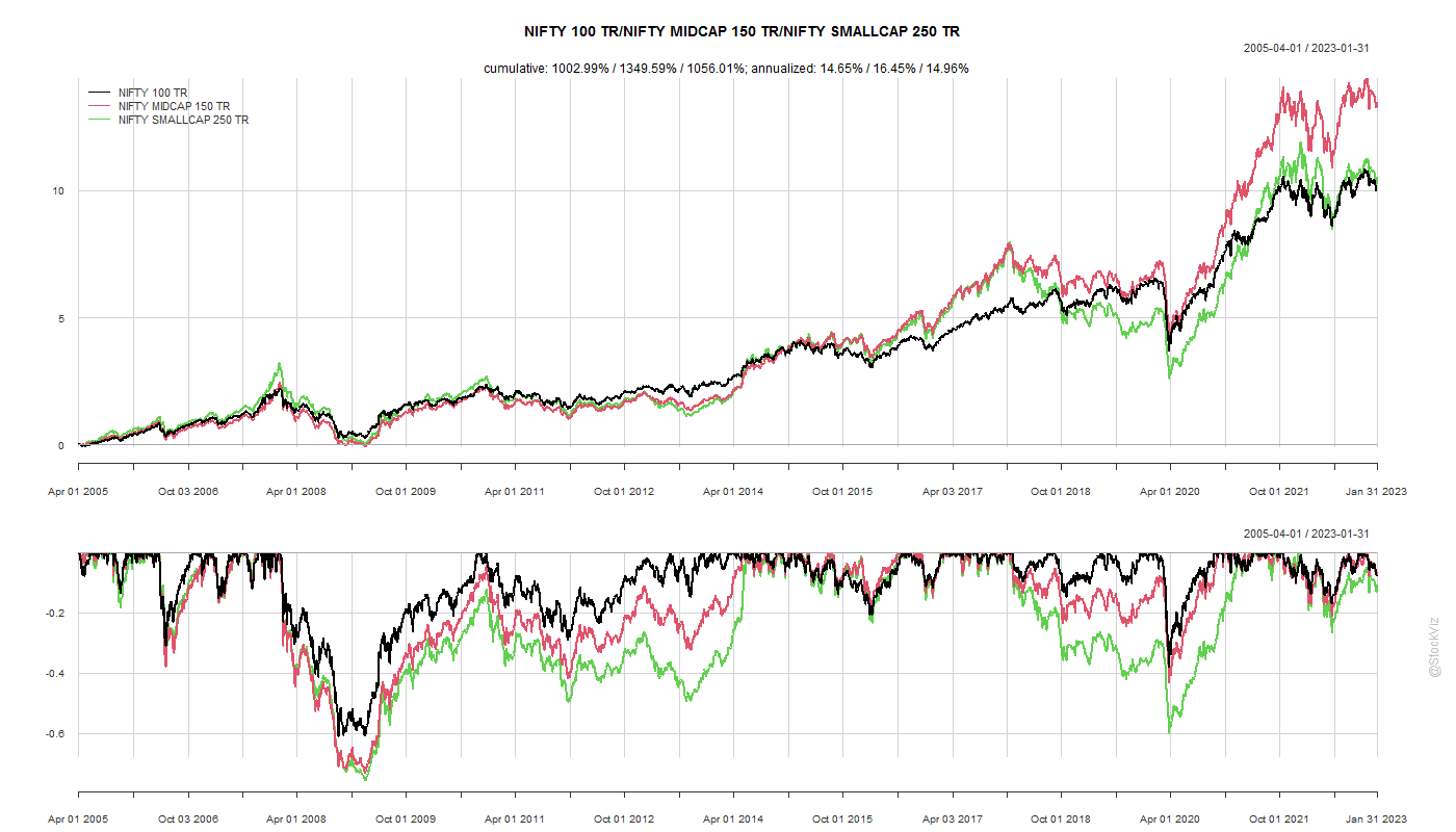
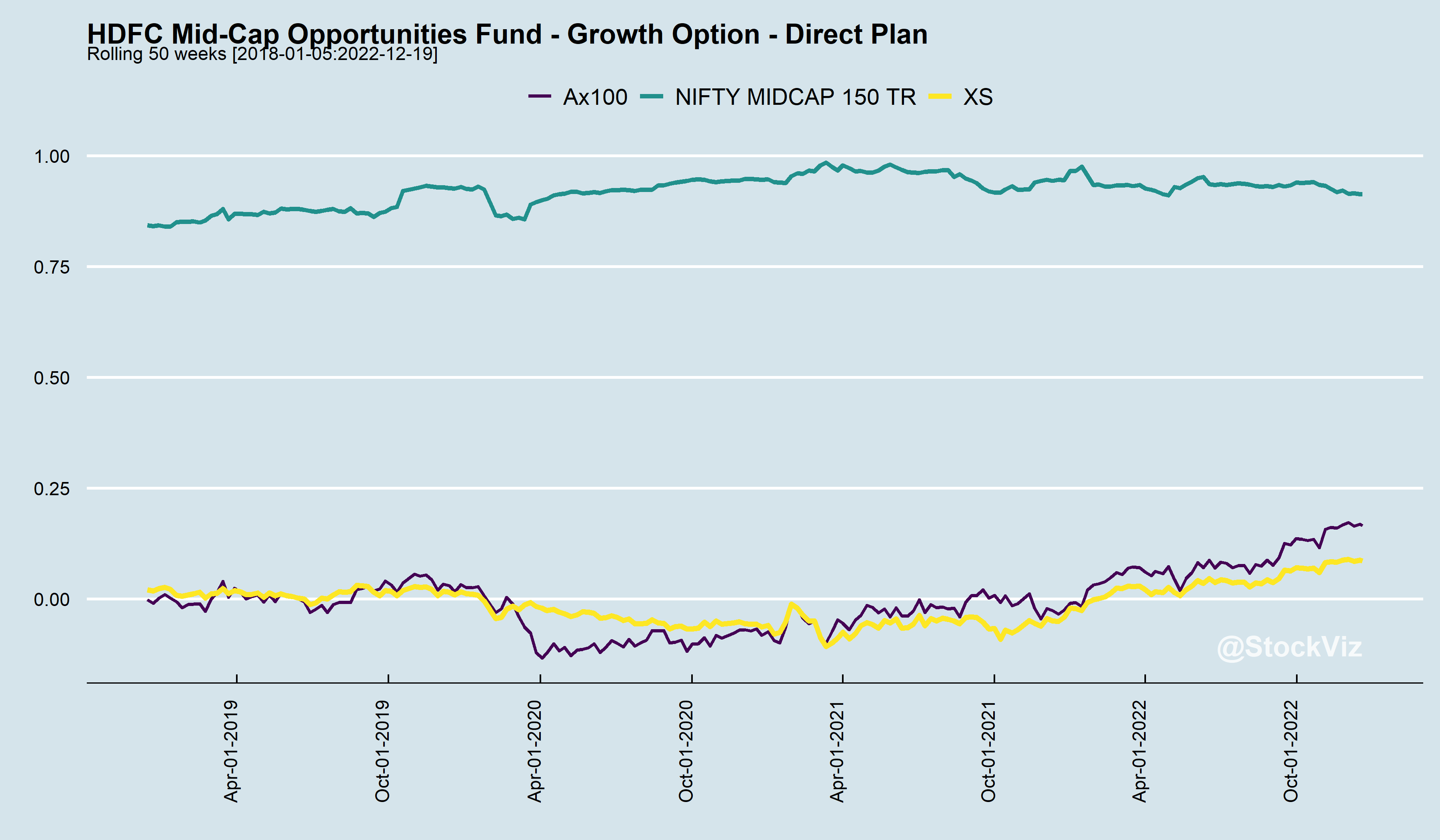
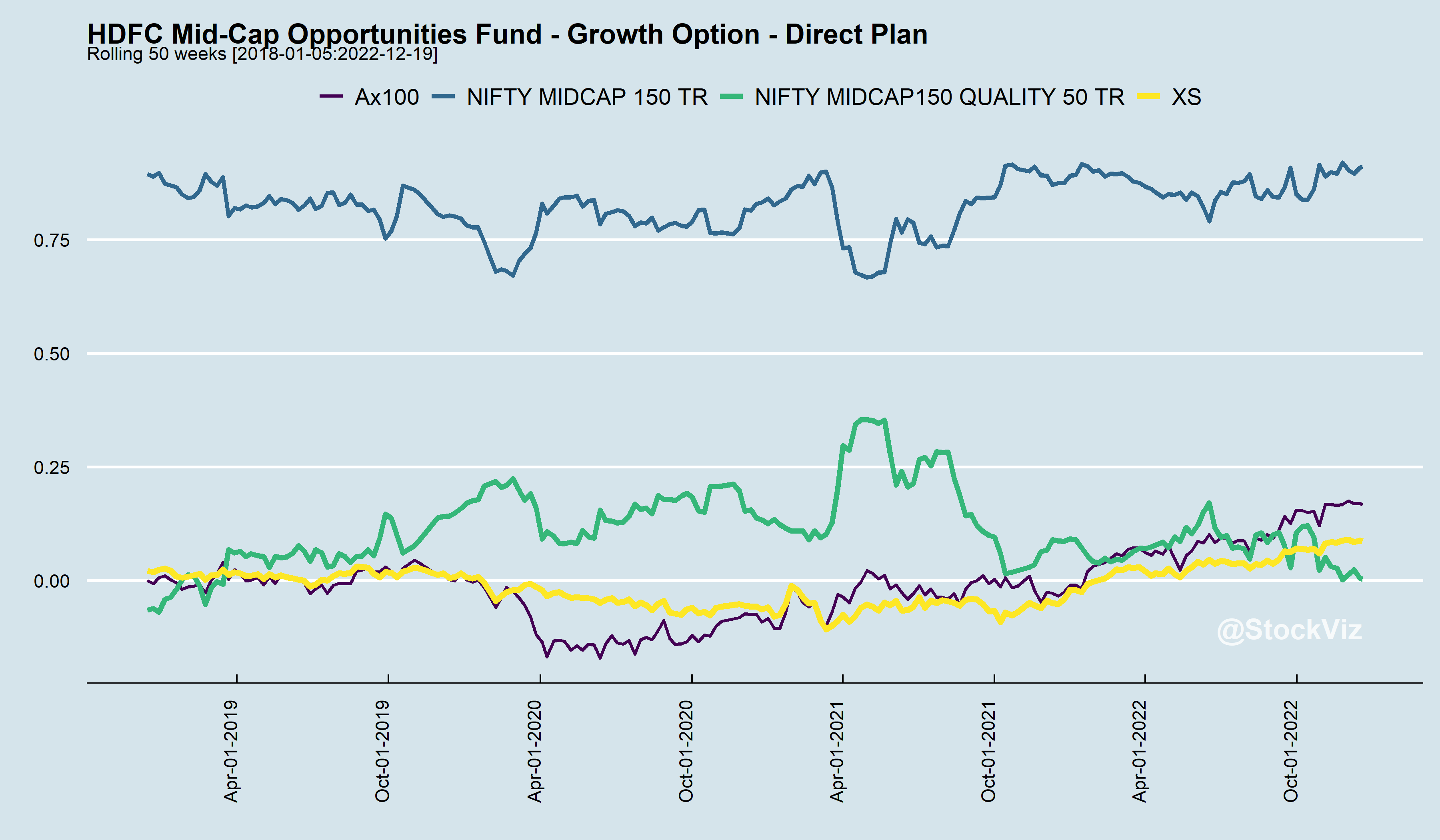
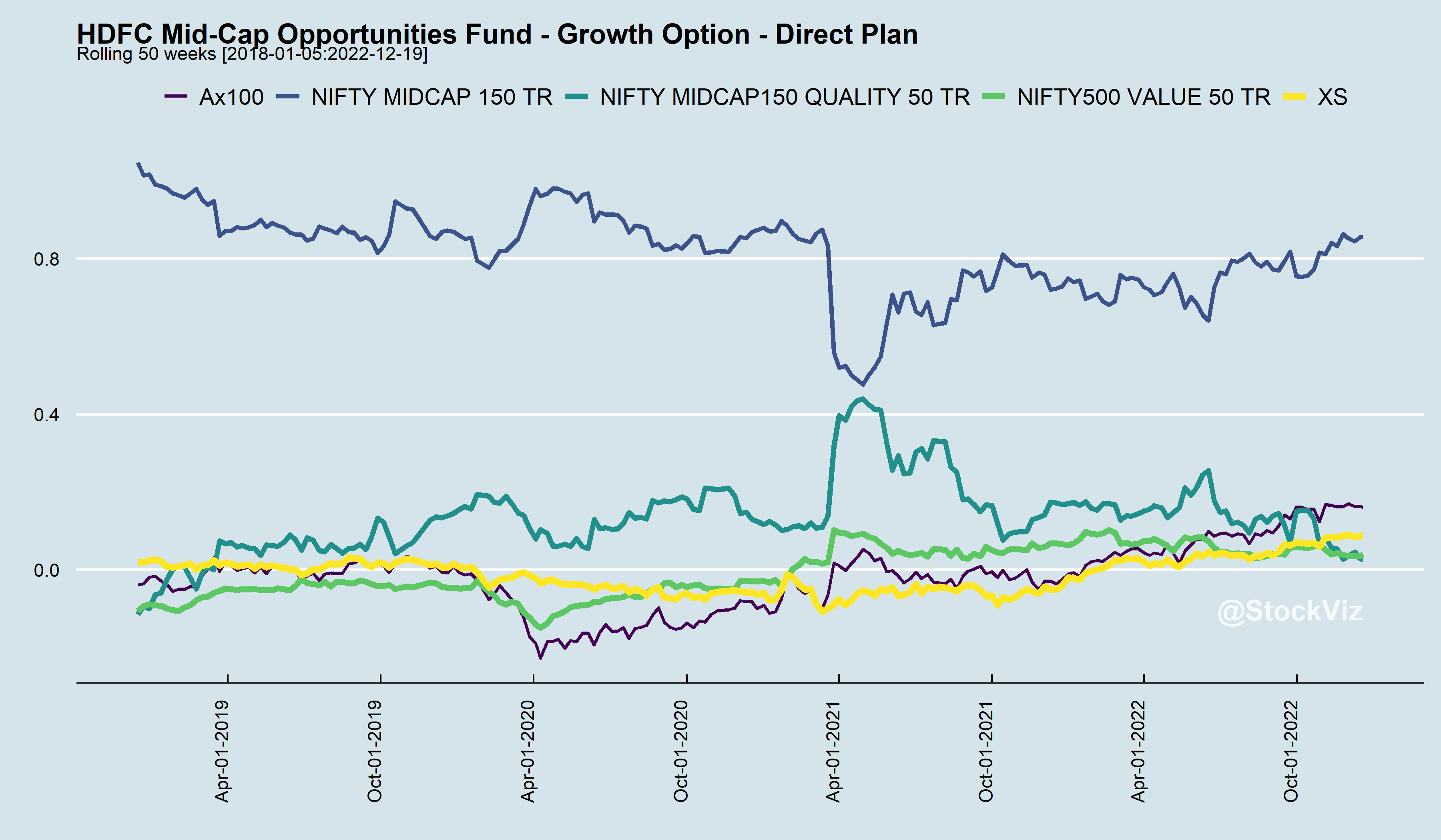
We took the basic intuition behind this and constructed a portfolio that switches between equities and bonds based on the Mahalanobis distance between them.
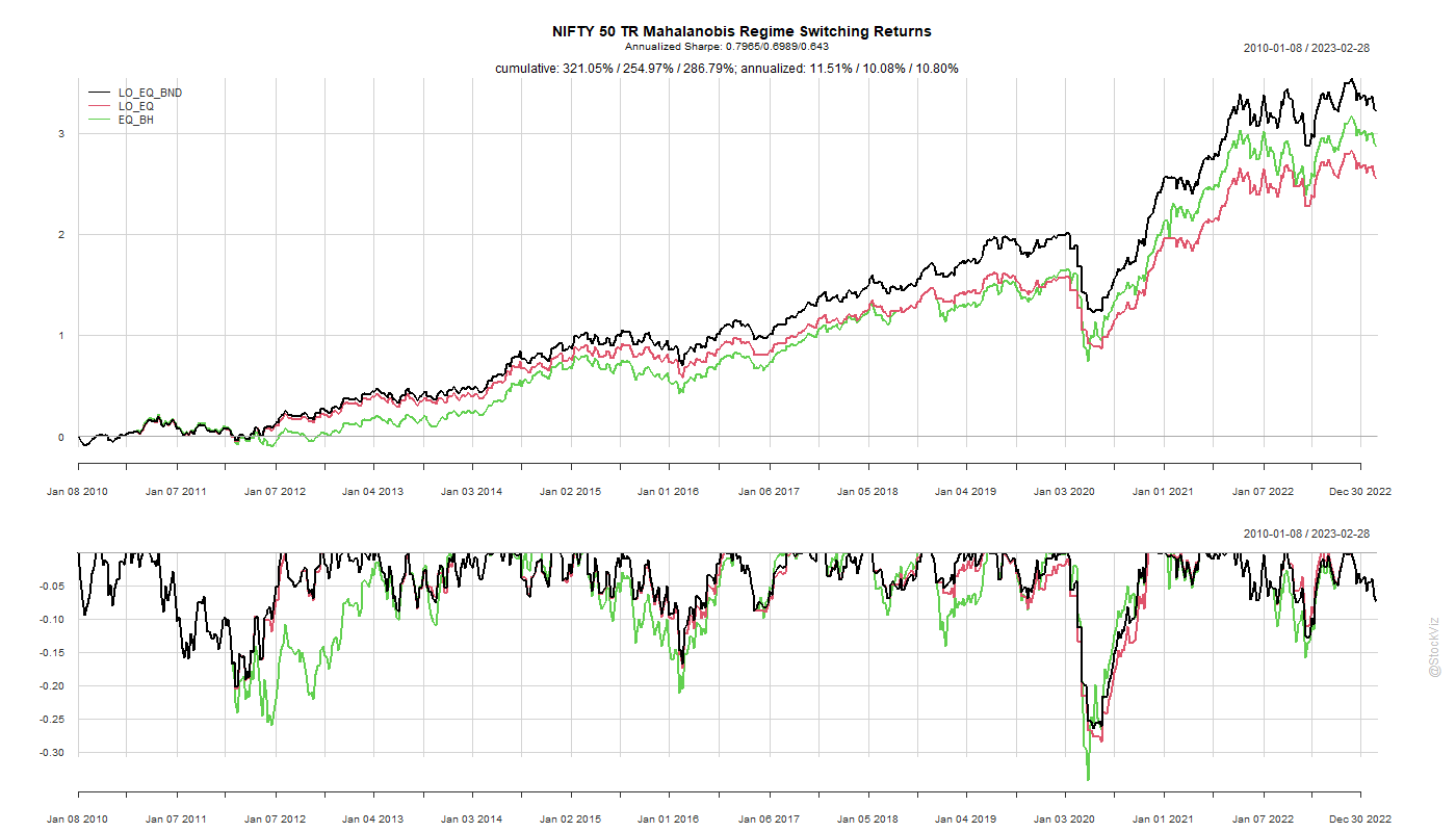
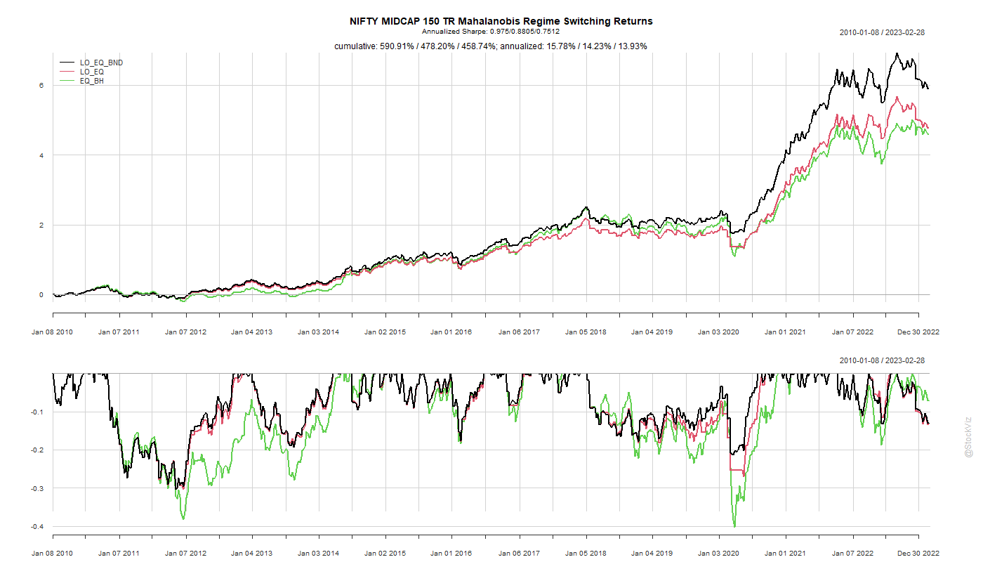
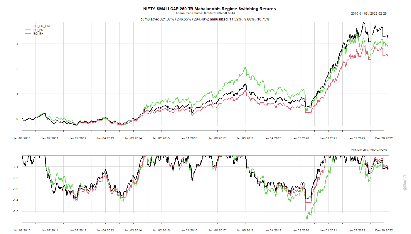
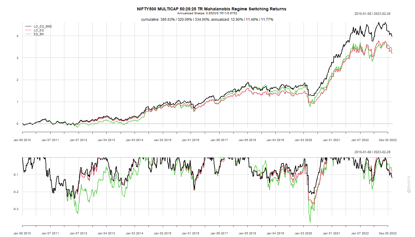
The out-of-sample results, factoring in transaction costs, look promising but doesn’t really stand out compared to other, more dumber, strategies that avoid steep drawdowns. However, two points over the Midcap buy & hold cannot be dismissed outright.
The code, charts and paper are on github.