Author: shyam

The High Volume Return Premium

Gervais, Simon, Ron Kaniel, and Dan H. Mingelgrin, 2001, “The high‐volume return premium,” The Journal of Finance, unearthed a market anomaly quite similar to momentum where stocks that traded with a higher than average volume went on to give higher returns.

We did a quick test on the top 200 stocks by free-float market cap on the NSE between 2014 and 2024 to check if it makes sense to pursue this further.

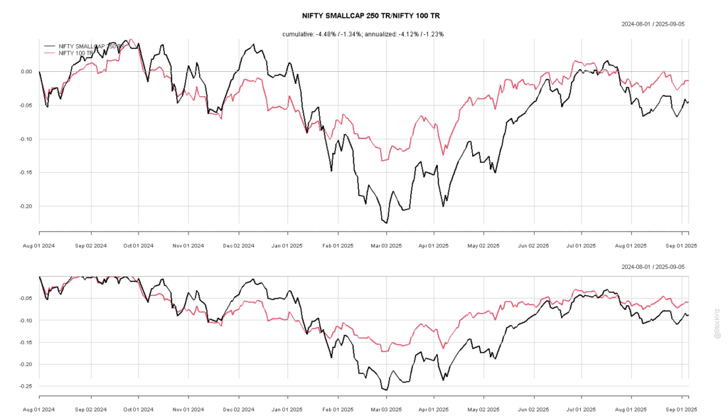
A long-only strategy that rebalanced once a month with a 50-day reference period underperformed the NIFTY 100 TR index by a wide margin until the August of 2023. Nine years of underperformance vs. a year of parabolic liftoff doesn’t really speak to the stability of the anomaly.

We’ll look for further publications in this area and report back. In the meantime, you can read the paper and have a look at our code here: github.

Commodities vs. Commodity Stocks

Trading commodities is not the same thing as trading commodity stocks. Commodity stocks, especially in partially-open economies like India, have their own cadence.

Take aluminum, for example. If you compare the MCX Aluminum Index with National Aluminum stock, the stock has vastly outperformed the metal.

While there is something to be said about the stock being more volatile than the metal, the difference is returns is night-and-day.

Stocks are evaluated on the basis of free-cashflow, earnings growth, return on capital, etc. While the prices of metals if mostly determined by short-term demand-supply imbalances.

Generally, Indian metal stocks have vastly outperformed the metals themselves.

If the government has erected tariff barriers to protect certain domestic industries, it makes no sense to try and link commodity prices to producer prices. Going back to our example, there is zero correlation between the monthly returns of aluminum vs. the monthly excess returns of National Aluminum (over the NIFTY 50 TR index) on any time frame.

Trading metals is completely different from trading metal stocks.

Code and charts on github.

Trends with (No) Benefits

It is easier to work with core strategies that fall into one of these extremes:

  1. low volatility / low max-drawdown that can be levered to achieve higher returns without blowing up, or
  2. high volatility / high max-drawdown and high returns that can be managed through asset-allocation and rebalancing.

The worst ones are those that have neither low volatility nor high returns.

Trend-following techniques deliver on (1). However, not everything trends.

Case in point are the Trendpilot ETFs PTLC over the S&P 500 (SPY) and PTNQ over the Nasdaq 100 (QQQ).

The methodology makes intuitive sense.

However, performance is a different matter.

The trend ETFs have worse Sharpe ratios than their benchmarks.

The silver lining is that the ETF versions are better than naïve trend strategies using only SMAs and would work out to be more cost and tax efficient than rolling your own.

However, the naïve versions all have Sharpe ratios less than 1.0 and high drawdowns. This tells us that the indices themselves may not amenable to trend-following and that they belong to (2) above?

Strategy design should follow the “first make it work then make it better” philosophy. If the simplest approach doesn’t work, then adding bells-and-whistles to it is unlikely to make it any better. If something is not trending, then what exactly are you following?

Code and charts are on github.

Trend Factor

Han, Yufeng and Zhou, Guofu and Zhu, Yingzi, A Trend Factor: Any Economic Gains from Using Information over Investment Horizons? (SSRN), outlines the construction of a trend factor for equities.

In this paper, we provide a trend factor that captures simultaneously all three stock price trends: the short-, intermediate-, and long-term, by exploiting information in moving average prices of various time lengths whose predictive power is justified by a proposed general equilibrium model. It outperforms substantially the well-known short-term reversal, momentum, and long-term reversal factors, which are based on the three price trends separately, by more than doubling their Sharpe ratios. 

Does the paper’s claim hold true for Indian equities? Not really.

The Long-only Trend Factor underperformed a naïve momentum strategy and its corresponding benchmark. The Long-short Trend factor returns was negative.

Even after “tuning” the look-back periods, the Trend Factor failed to beat momentum.

Constructing a portfolio of stocks using trend following seems to be a dead end. Our previous attempts at this — Dynamic Linear Model v1.0 and Dynamic Equity Trend-following — have yielded similar results as well.

Momentum beats Trend-Following.

Code and charts are on github.

SVM for Momentum

Previously, we explored if Meta’s Prophet library could be used to drive a momentum portfolio (Prophet for Momentum, Prophet for Momentum, Part II). We found that a simple (naïve) momentum strategy outperformed whatever we did with Prophet.

More generally, using a Neural Network or an SVM to drive portfolios have been a disappointment in live scenarios (Machine Learning Themes). Their after cost performance trail benchmarks.

Moreover, a big problem with these models is that there are a million different ways to specify them and a few of them will go on to outperform in a forward-test simply because they load on a factor that is working for that moment in time. So, you never know if you found the “right” set of specs (because there is none) and if you are not careful, you will forever be tuning the model based on what worked in the recent past.

Even simple SVMs come with so many different ways to specify them: classification vs. regression, polynomial degree, cost (static vs. auto-tune), feature selection, feature tuning, etc. And, since we don’t know which ones work beforehand, we try most of them and settle on those specs that output the results we wanted.

For example, an SVM can be trained with a time-series of previous month’s returns to predict the next month’s returns. A momentum portfolio can be created by ranking these predictions. Rebalance every month and you have something that works.

The problem is that to arrive at this model, we went through a fair amount of parameter and feature tweaking/tuning which may or may not work in the future.

Here, we published the charts of an SVM that uses a 5th degree polynomial kernel because it worked (higher Sharpe!) and not because there is a strong theoretical reason why 5 is better than 1.

For every model that is published, be rest assured that there are thousands hidden away in a drawer.

This is why we remain skeptical of “A.I.” investment strategies.

Code and charts on github.