Author: shyam

Monitoring Network Glitches

More often than not, real time feeds are exposed as web socket streams. Web sockets are extremely sensitive to network glitches. Glitches – when the connection drops for a very small span of time – will cause your market data to lag badly as your client tries to reconnect/re-establish the feed, eventually leading to catastrophic failure.

The problem with glitches is that it is hard to work around. A complete drop in the connection can be handled by a router that can switch over to a backup connection. Glitches are more sinister.

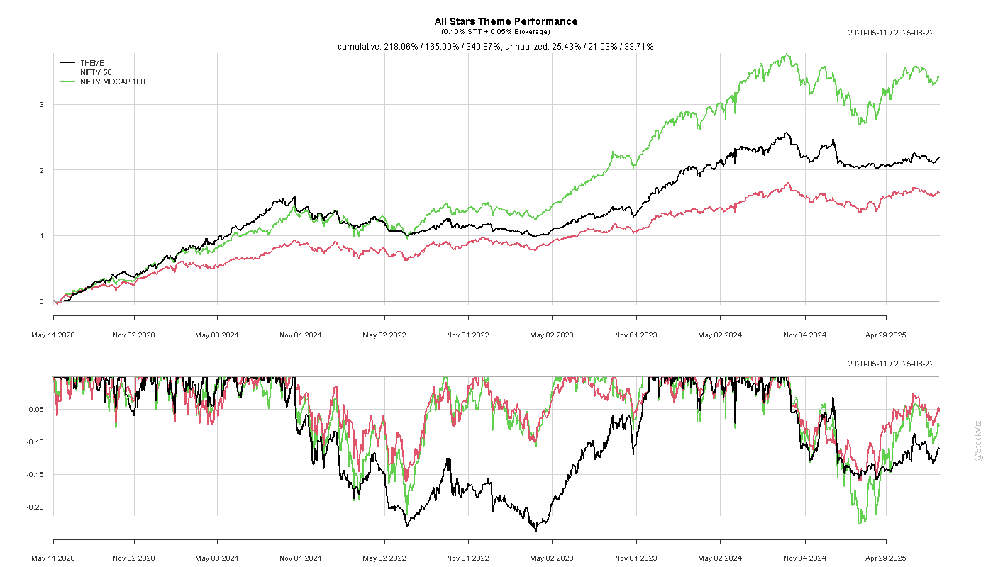
For example, we have broadband connections from three different service providers (Hathway, Excitel and BSNL) to make sure our systems can stay connected. They all have varying degrees of stability and customer service. Here are the number of glitches per hour over the last few days:

You can work around 1-2 glitches an hour by making your re-connection logic more robust. However, there is no getting around the Hathway level of glitches.

If your service provider itself is not monitoring for glitches, then explaining the problem to them is impossible. Support tickets get closed because “network is connected.” Here is a history of our support tickets with Hathway – an ongoing saga with no end:

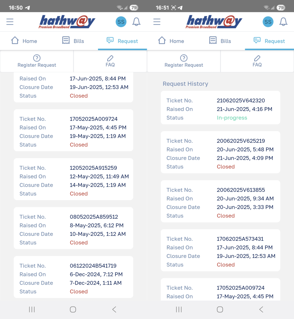
As you scale, monitoring your infrastructure becomes increasingly important. Be aware that your service provider could be (willfully) blind to the specific issues you are facing – their job might depend on them not solving it. And, always have a backup and a backup for your backup.

The python code to monitor for glitches and the R code to draw the charts are on github.

Momentum Skip Month (II)

Our earlier post on using a “skip” month for setting up momentum portfolios saw a slight advantage in skipping a month. However, it very will could have been because of path dependence.

Going back to a 20-stock portfolio and separating out the monthly returns of stocks only in the “no-skip” portfolio (RET_NOSKIP) and those that are only in the one-month skipped portfolio (RET_SKIP) doesn’t really settle the debate in favor of skipping a month.

The summary stats are similar as well.

Perhaps the mean reversion that was observed prior to the early 90’s when the original paper was published is weaker now?

Code on github.

Volatility as Beta

The volatility risk premium (VRP) is the difference between implied volatility and realized (or actual historical) volatility. Implied volatility is, on average, overpriced compared to realized volatility.

The VRP exists because investors are essentially “selling insurance” when they sell implied volatility.

Volatility is negatively correlated with equity returns; typically, volatility increases when equity markets decline. Therefore, a short volatility position is implicitly “long equity risk”. Since equities are generally expected to earn an equity risk premium (ERP) over the risk-free rate, strategies that are implicitly long equity risk should also be abnormally profitable. This is why short volatility strategies tend to be profitable on average.

Just like how you can get long ERP by getting long an equity index, you should be able to get long VRP by programmatically shorting options and delta-hedging them. Volatility becomes a beta that you allocate towards.

Building Blocks

An option’s value changes relative to the price of the underlying – the rate of this change is called delta.

Gamma is the rate of change of delta given a change in the price of the underlying. As the underlying price moves, an option’s delta does not remain constant; gamma quantifies how much that delta will change.

Since we are only interested in volatility and not price, we can hedge out this delta. Delta-hedging a basket of options mitigates the exposure to the directional movement of the underlying. Profitability becomes solely determined by the volatility (not direction) of the underlying.

Vega is the rate of change of an option’s value relative to a change in implied volatility (IV). If IV rises or declines by one percentage point, the value of the option is expected to rise or decline by the amount of the option’s vega, respectively.

When you short options, you have negative gamma (you don’t want large price movements) and negative vega (you don’t want IV to rise). You hope for low realized volatility and falling IV. However, you have positive theta — time works in your favor.

Theoretically, a delta-hedged short option position’s P&L = vega(IV – RV).1

Construction

Historically, NIFTY ATM option Implied Volatility across days-to-expiry, looks like this:

So, theoretically, if you shorted 30dte ATM calls and exited them at 7dte, your P&L distribution will look like this:

And the same thing with puts:

If you are willing to treat volatility as just-an-other beta, then by creating programmatic delta-hedged short ATM straddle/strangle portfolio, you can get long this beta.

Just as it is with ERP, one could build models to time VRP. Having a beta portfolio as a benchmark should help.

  1. Volatility Trading, Euan Sinclair ↩︎

Bitcoin Volatility Seasonality

Is Bitcoin Volatility seasonal? Yes.

There are calm months and there are frantic ones…

When you decompose the series, you can see the ebb and flow of monthly seasonality.

The pattern largely holds post-COVID as well — even after Bitcoin began its journey as an institutionally accepted asset.

Zooming in on the seasonal component alone, you can see how it troughs around October-November.

And this has tracked post-COVID as well.

The seasonal component has been negative during the months of July through December indicating that the volatility experienced during that time was idiosyncratic.

Code and charts on github.

Related: INDIA VIX Seasonality

Buy Highs/Sell Lows

In equities, buying stocks that hit their All Time Highs is a decent strategy. When combined with a trailing stop loss, it beats the NIFTY 50 index with a Sharpe of around 1.8.

Can a similar long/short strategy work in crypto?

Since everything happens faster in crypto, we need to relax the “All-Time” constraint and consider shorter time-frames. For example, here’s the 200-day Highs stats, for returns of subsequent 1/5/10 & 20 days of L1 and L2 coins:

And here’s the same for 20-day Highs stats:

A similar thing plays out with 200- and 20-day lows.

Theoretically, you can go long coins making 20/50-day highs and go short coins making 20/50-day lows. Apply a reasonable trailing stop loss and you might have a decent strategy.

Code and charts on github.