Transfer Entropy

In investing, we are always trying to find the relationship between two entities. For example, to hedge a long portfolio, we typically calculate the “beta” with respect to an index and use that to go short the index. Here, the biggest assumption is that the relationship is linear (or at least, piecewise linear.)

However, relationships in finance are typically non-linear. Using the math behind calculating entropy is one way to overcome the “beta” problem.

Introduction

From Wikipedia: Transfer entropy is a non-parametric statistic measuring the amount of directed (time-asymmetric) transfer of information between two random processes.

It tries to answer a simple question: what the effect of one entity over another, given a lag?

From StackExchange: TE(X↦Y)=0.624 means that the history of the X process has 0.624 bits of additional information for predicting the next value of Y. (i.e., it provides information about the future of Y, in addition to what we know from the history of Y). Since it is non-zero, you can conclude that X influences Y in some way.

Quick Look

Luckily, both R and python have libraries that help calculate transfer entropies between two variables.

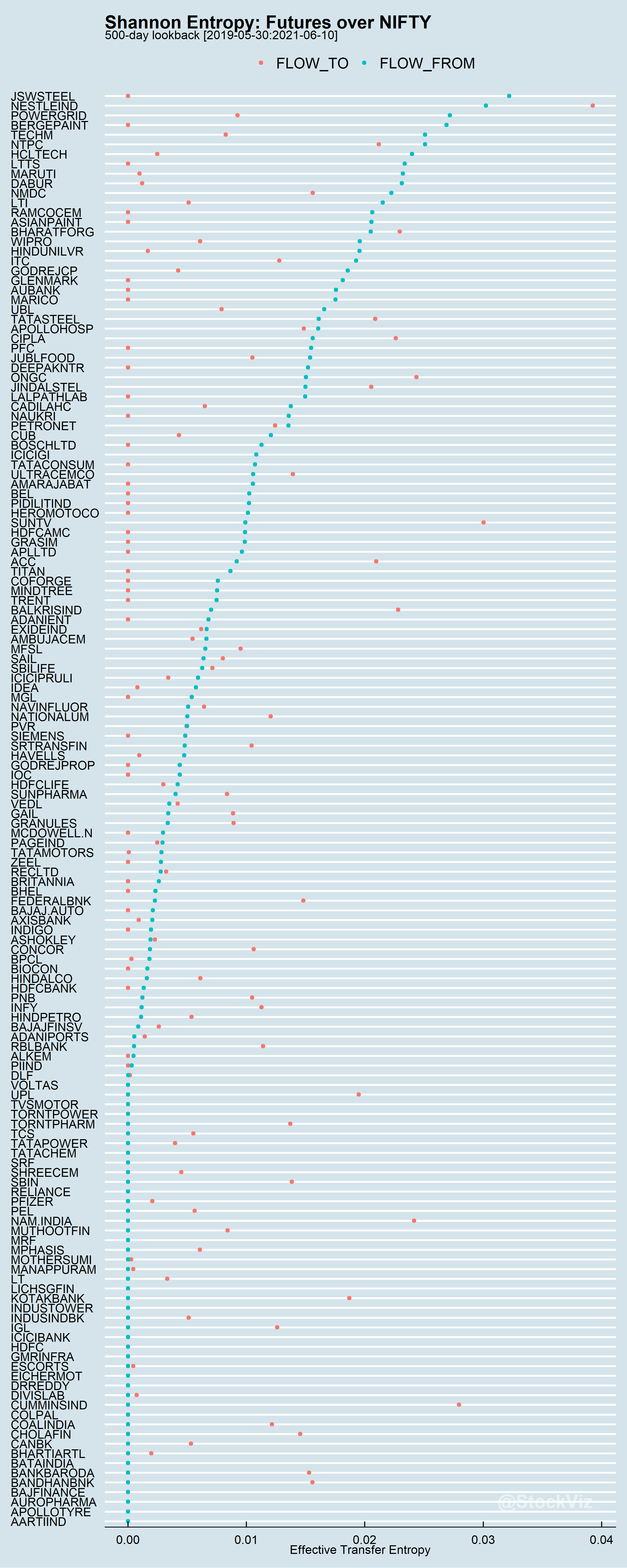
Here’s the TE between Stock Futures and the NIFTY with a 500 day lookback and a single-day lag. FLOW_TO is a measure of information flow from the stock to the index and FLOW_FROM is the opposite direction.

Next Steps

This has interesting applications in portfolio risk management. Instead of calculating beta and hoping for the best, we could use TE to get a better understanding of how the individual constituents are affected by the index and hedge only those that have large values.

This post was inspired by Concepts of Entropy in Finance: Transfer entropy. Code and images for this post are on Github.